Graph clustering with SBM

Loads packages and set a future plan for parallel processing if you want.

library(future)
library(Matrix)
library(ggplot2)
library(greed)

Simulation of an SBM graph with a hierarchical structure.

N=400
K=6
pi=rep(1/K,K)
lambda  = 0.1
lambda_o = 0.01
Ks=3
mu = bdiag(lapply(1:(K/Ks), function(k){matrix(lambda_o,Ks,Ks)+diag(rep(lambda,Ks))}))+0.001
sbm = rsbm(N,pi,mu)

Perform the clustering with default model and algorithm. We specify to choose an sbm model since for squared sparse matrix the default is a DcSbm model. An hybrid algorithm is selected by default and the default value for the parameter K is 20.

sol = greed(sbm$x,model = Sbm())
#> ------- guess SBM model fitting ------
#> ################# Generation  1: best solution with an ICL of -14174 and 6 clusters #################
#> ################# Generation  2: best solution with an ICL of -14174 and 6 clusters #################
#> [1] "clean ok"
#> ------- Final clustering -------
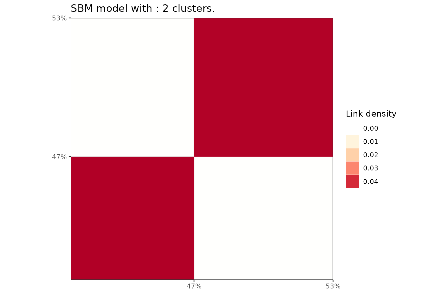
#> ICL clustering with a SBM model, 6 clusters and an icl of -14174.

Plot the results using a block representation.

plot(sol,type='blocks')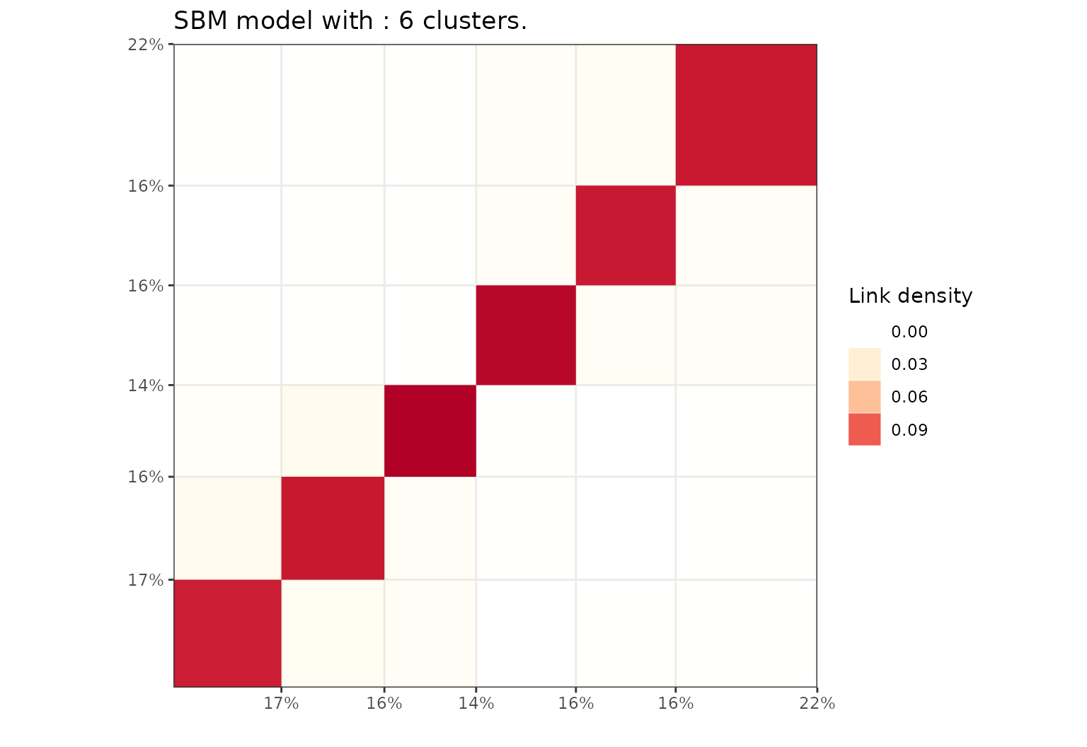

Plot the results with a node link diagram.

plot(sol,type='nodelink')

Or a dendrogram for selecting a smaller value for K.

plot(sol,type='tree')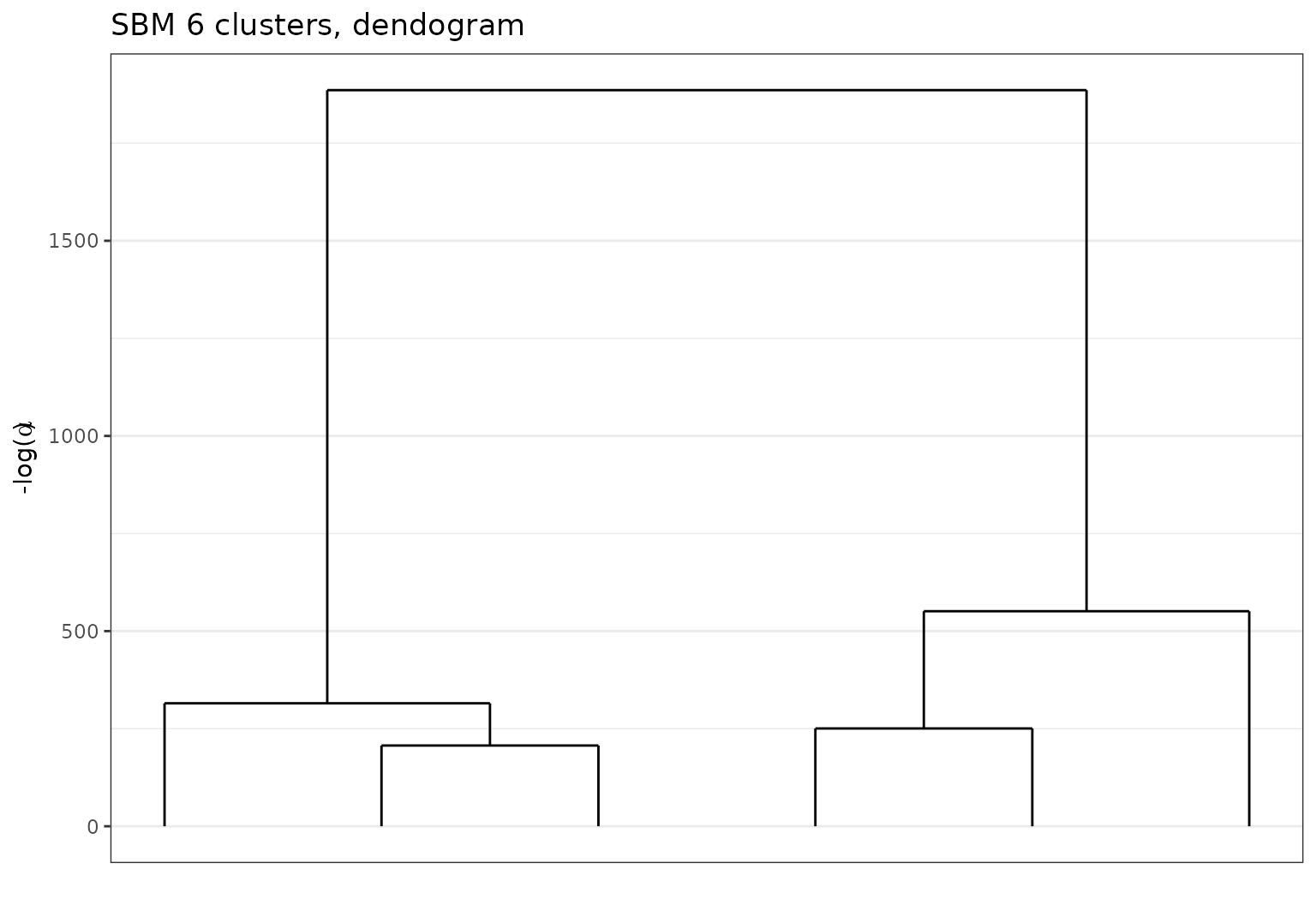

Eventually study the evolution of \(-log(\alpha)\) with respect to \(K\).

plot(sol,type='path')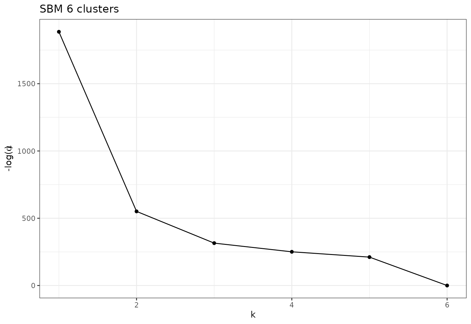

Or of ICL with respect to \(log(\alpha)\)

plot(sol,type='front')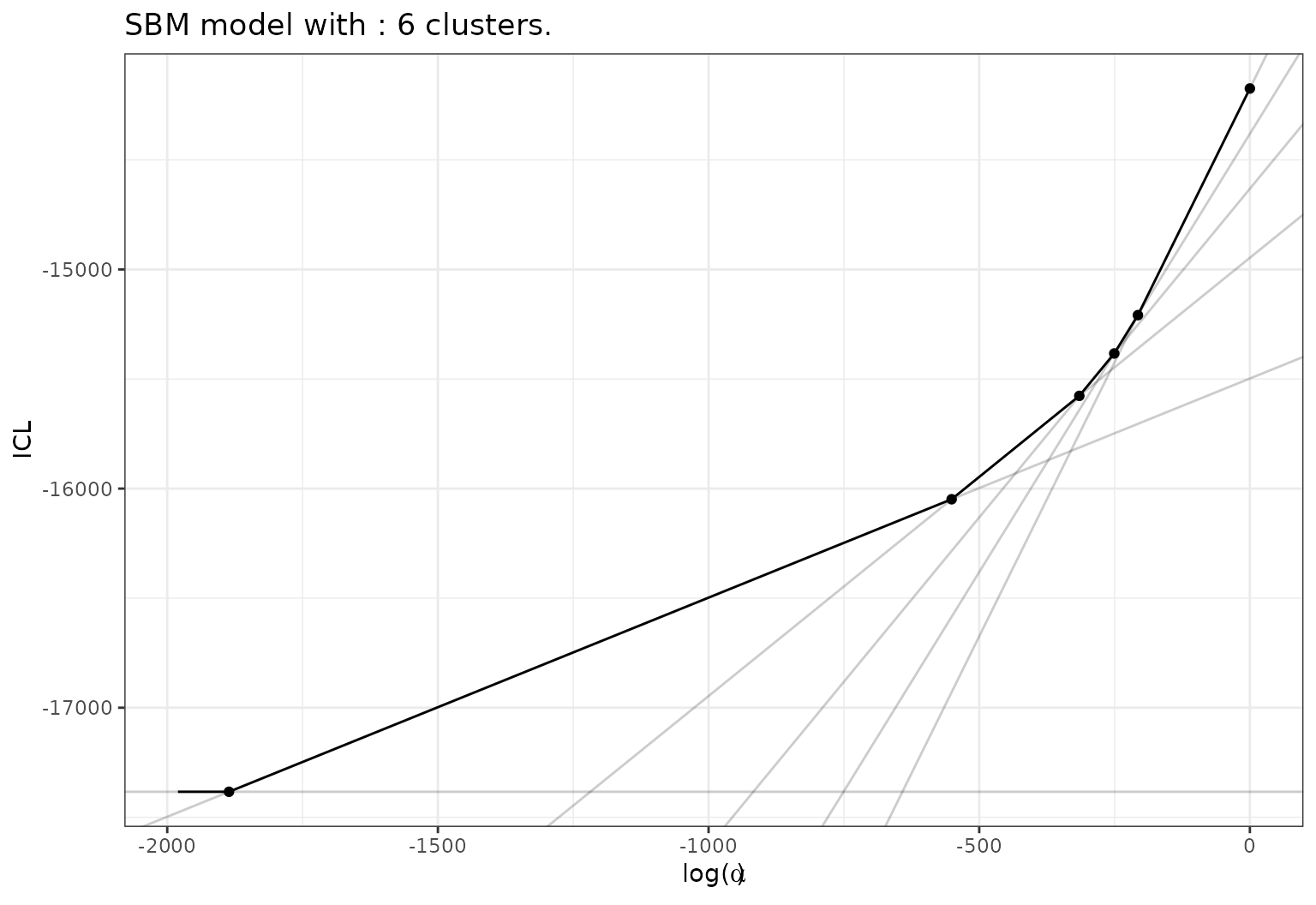

And select a smaller value to extract a new solution.

sol2 = cut(sol,2)
plot(sol2,type='blocks')

Etienne Côme

2021-11-19