Continuous data clustering with Gaussian mixtures

Etienne Côme & Nicolas Jouvin

Loads packages.

library(future) # allows parralel processing in greed()
library(greed)
library(dplyr)
library(ggplot2)
set.seed(2134)

future::plan("multisession", workers=2) # may be increased 

The model

Gaussian Mixture Models (GMMs) count among the most widely used DLVMs for continuous data clustering. The greed package handles this family of models and implements efficient visualization tools for the clustering results that we detail below.

Without any constraints, the Bayesian formulation of GMMs leading to a tractable exact ICL expression uses a Normal and inverse-Wishart conjugate prior on the mean and covariances \(\mathbf{\theta} = (\mathbf{\mu}_k, \mathbf{\Sigma}_k)_k\). This prior is defined with hyperparameters \(\mathbf{\beta} = (\mathbf{\mu}, \tau, n_0, \mathbf{\varepsilon})\) and the hierarchical model is written as follows:

\[\begin{equation} \label{eq:gmm} \begin{aligned} \pi&\sim \textrm{Dirichlet}_K(\alpha)\\ Z_i&\sim \mathcal{M}(1,\pi)\\ \mathbf{\Sigma}_k^{-1} & \sim \textrm{Wishart}(\mathbf{\varepsilon}^{-1},n_0)\\ \mathbf{\mu}_k&\sim \mathcal{N}(\mathbf{\mu},\frac{1}{\tau} \mathbf{\Sigma}_k)\\ X_{i}|Z_{ik}=1 &\sim \mathcal{N}(\mathbf{\mu}_k, \mathbf{\Sigma}_{k})\\ \end{aligned} \end{equation}\]

Contrary to other models, these priors are informative and may therefore have a sensible impact on the obtained results. By default, the priors parameters are set as follow:

• \(\alpha=1\)
• \(\mu=\bar{X}\)
• \(\tau=0.01\)
• \(n_0=d\)
• \(\mathbf{\varepsilon}=0.1\,\textrm{diag}(\mathbf{\hat{\Sigma}}_{\mathbf{X}})\)

These default values were chosen to accommodate a variety of situation but may be modified easily. For more details, we refer to the class documentation ?Gmm. Finally, it is possible to specify constraints on the covariance matrix as discussed below.

An introductory example : the diabetes dataset

Let us describe a first use case on the diabetes dataset from the mclust package. The data describes \(p=3\) biological variables for \(n=145\) patients with \(K=3\) different types of diabetes: normal, overt and chemical. We are interested in the clustering of this dataset to see if the three biological variables can discriminate between the three diabetes type.

data(diabetes,package="mclust")
X=diabetes[,-1]
X = data.frame(scale(X)) # centering and scaling

Clustering with greed and GMM

We apply the greed() function with a Gmm object with default hyperparameters. The optimization algorithm used by default is the hybrid genetic algorithm of Come et. al (2021).

sol = greed(X,model=Gmm())
#> 
#> ── Fitting a GMM model ──
#> 
#> ℹ Initializing a population of 20 solutions.
#> ℹ Generation 1 : best solution with an ICL of -288 and 6 clusters.
#> ℹ Generation 2 : best solution with an ICL of -264 and 3 clusters.
#> ℹ Generation 3 : best solution with an ICL of -264 and 3 clusters.
#> ── Final clustering ──
#> 
#> ── Clustering with a GMM model 3 clusters and an ICL of -264

The optimal clustering found by the hybrid GA has \(K^\star=3\) clusters. You may then easily extract the found clustering with the clustering() method and compare it with the known classes:

table(diabetes$cl,clustering(sol)) %>% knitr::kable()

	1	2	3
Chemical	0	24	12
Normal	0	2	74
Overt	26	7	0

It roughly corresponds to the known groups with cluster 1,2 and 3 recovering overt, chemical and normal diabetes respectively, with some miss-classifications that are expected with GMM clustering on this dataset.

To get an overview of the clustering results, you may also use the gmmpairs() plot function which displays the scatter plot matrix, colored by cluster membership, with estimated Gaussian ellipses in each cluster via maximum a posteriori:

gmmpairs(sol,X)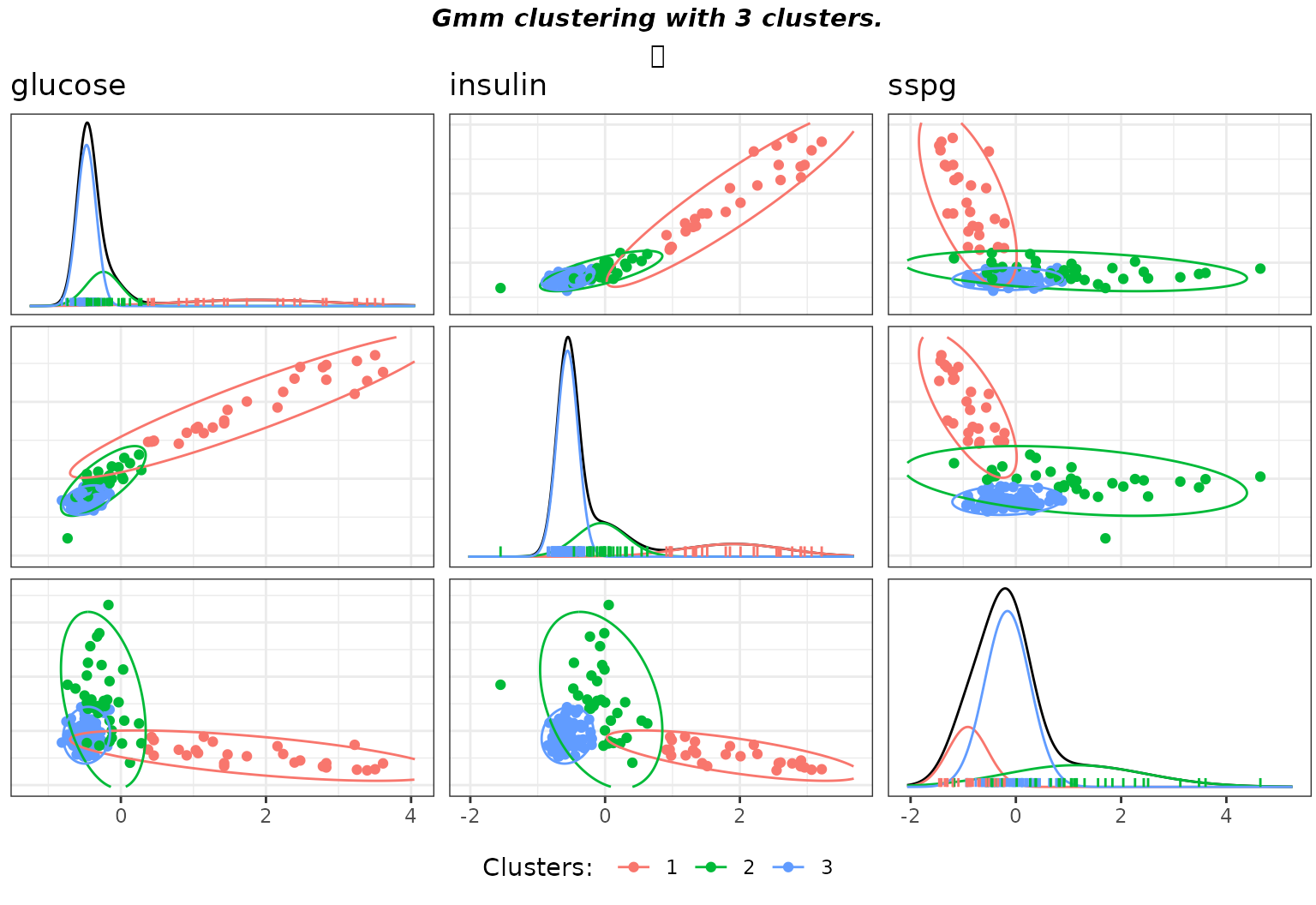 

Matrix pairs plots of the clustering with default hyperparameters on the diabetes data.

Furthermore, users may use the generic coef() function to get the mixture component parameters, or rather their maximum a posteriori estimated conditionally on the partition. The result will be a simple list with fields for each parameters (means: muk, covariance matrices: Sigmak, proportions: pi). Here is an example for the \(3\)-component GMM we just extracted, were we extract the mean of the first component.

params = coef(sol)
names(params)
#> [1] "pi"     "muk"    "Sigmak"
params$muk[[1]]
#>       glucose  insulin      sspg
#> [1,] 1.871123 1.914675 -0.912741

If a user wants to experiment with other values of the prior hyperparameters, the most important is \(\mathbf{\varepsilon}\), which control the clusters’ covariance matrices Wishart prior. This amounts to specify the prior on the dispersion inside each class. For instance, one may specify a priori belief that the variance is small inside clusters, which amounts to diminish the \(0.1\) coefficient in front of \(\hat{\mathbf{\Sigma}}_{\mathbf{X}}\). In this case, it makes sense to decrease \(\tau\) in the same proportions to keep a flat priors on the clusters means. For the diabetes data such a choice leads to an interesting solution, where the strong prior constraint leads to one cluster being created to fit one outlier in the “chemical” diabetes.

sol_dense = greed(X,model=Gmm(epsilon=0.01*diag(diag(cov(X))), tau =0.001))
#> 
#> ── Fitting a GMM model ──
#> 
#> ℹ Initializing a population of 20 solutions.
#> ℹ Generation 1 : best solution with an ICL of -372 and 12 clusters.
#> ℹ Generation 2 : best solution with an ICL of -328 and 7 clusters.
#> ℹ Generation 3 : best solution with an ICL of -306 and 5 clusters.
#> ℹ Generation 4 : best solution with an ICL of -306 and 5 clusters.
#> ── Final clustering ──
#> 
#> ── Clustering with a GMM model 3 clusters and an ICL of -304
gmmpairs(sol_dense,X)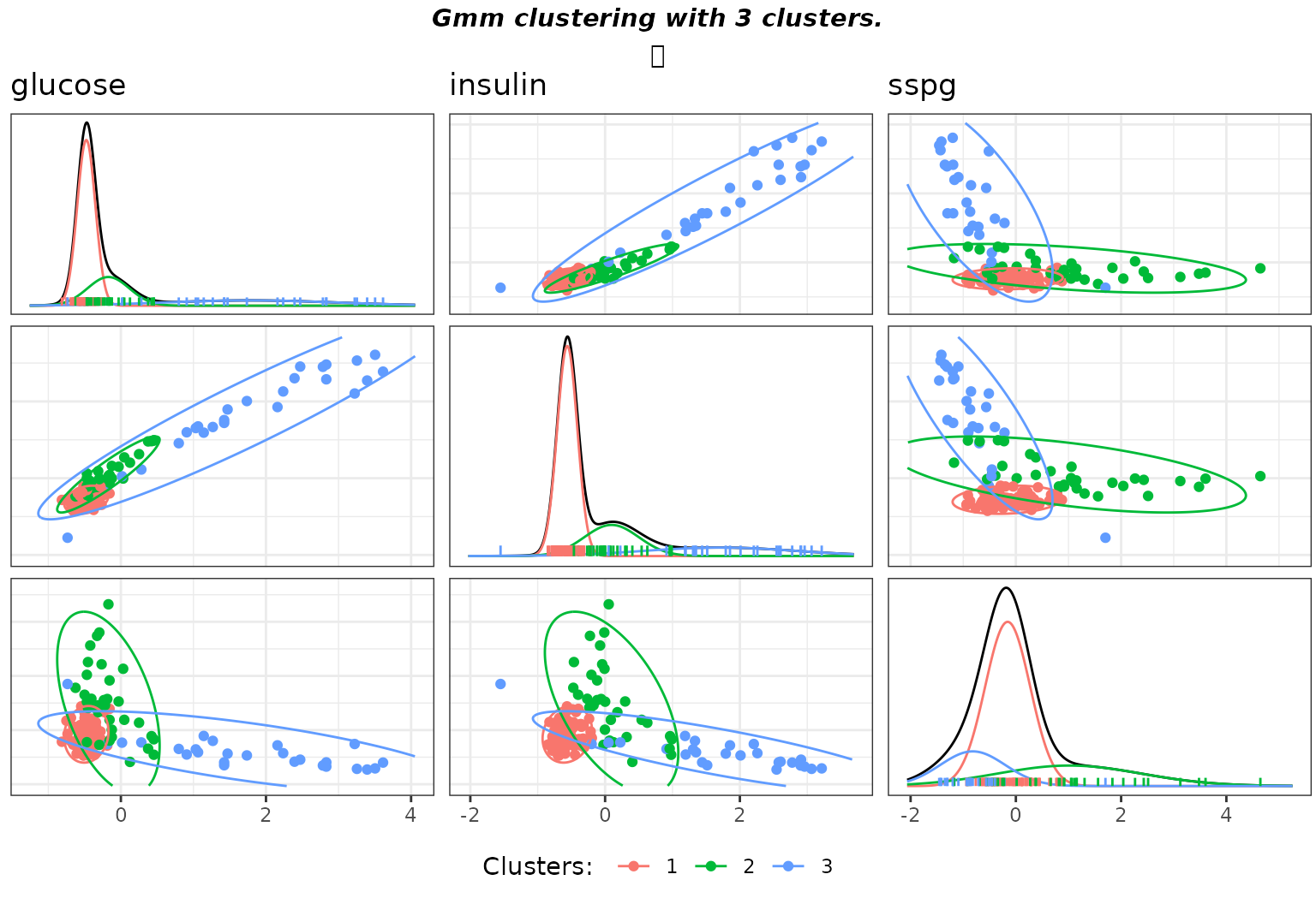

Matrix pairs plots of the clustering with user specified hyperparameters on the diabetes data.

Diagonal covariance matrix

When the number of variables \(p\) becomes large, it can be of interest to reduce the flexibility of a GMM by adding a specific set of constraints. The diagonal covariance model, with constraint \(\mathbf{\Sigma}_k = \textrm{diag}(\sigma_{k1}, \ldots, \sigma_{kp})\), is implemented in the greed package through its DiagGmm S4 class. Its hierarchical formulation is similar to unconstrained GMM, except the Wishart prior on \(\mathbf{\Sigma}_k\) is now replaced by a Gamma prior on each \(\sigma_{kj}\) with shape \(\kappa\) and rate \(\beta\) hyperparameters defaulted to \(1\) and mean of the empirical columns variances respectively.

Fitting this model on the diabetes dataset, greed() with an hybrid GA finds a \(4\)-components diagonal GMM.

soldiag = greed(X,model=DiagGmm())
#> 
#> ── Fitting a DIAGGMM model ──
#> 
#> ℹ Initializing a population of 20 solutions.
#> ℹ Generation 1 : best solution with an ICL of -292 and 6 clusters.
#> ℹ Generation 2 : best solution with an ICL of -285 and 6 clusters.
#> ℹ Generation 3 : best solution with an ICL of -285 and 6 clusters.
#> ── Final clustering ──
#> 
#> ── Clustering with a DIAGGMM model 5 clusters and an ICL of -279
gmmpairs(soldiag,X)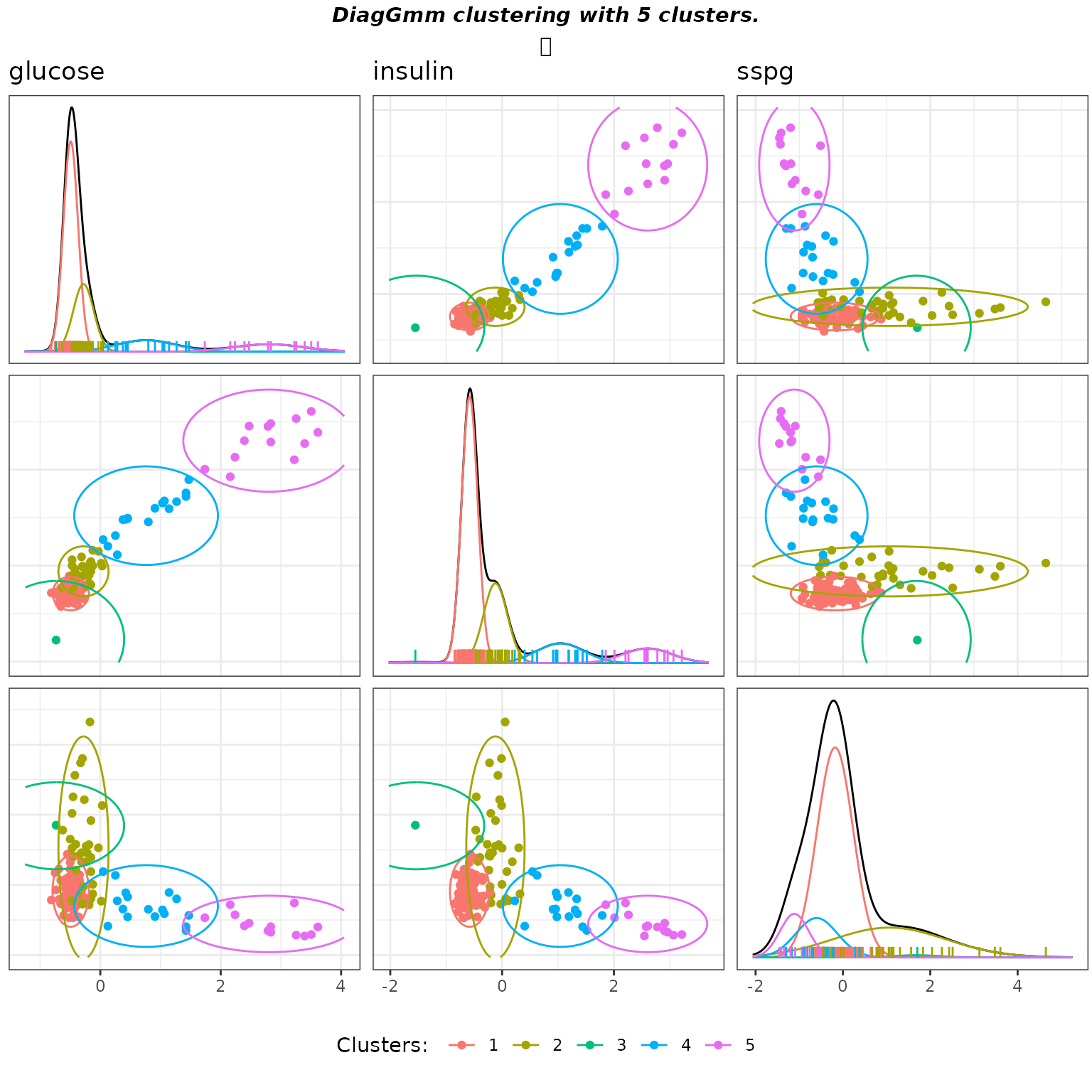

Matrix pairs plots of the Diagonal GMM clustering with default parameters on the diabetes data.

As previously, the clustering is quite aligned with the known groups except that now two clusters were needed to fit the “overt” class which presents an important elongation.

table(diabetes$cl,clustering(soldiag)) %>% knitr::kable()

	1	2	3	4	5
Chemical	8	27	1	0	0
Normal	71	5	0	0	0
Overt	0	3	0	17	13

Moreover, we may investigate coarser partitions when inspecting a clustering. To plot the dendogram, one may simply use the plot function with the type option set to 'tree':

plot(soldiag,type='tree')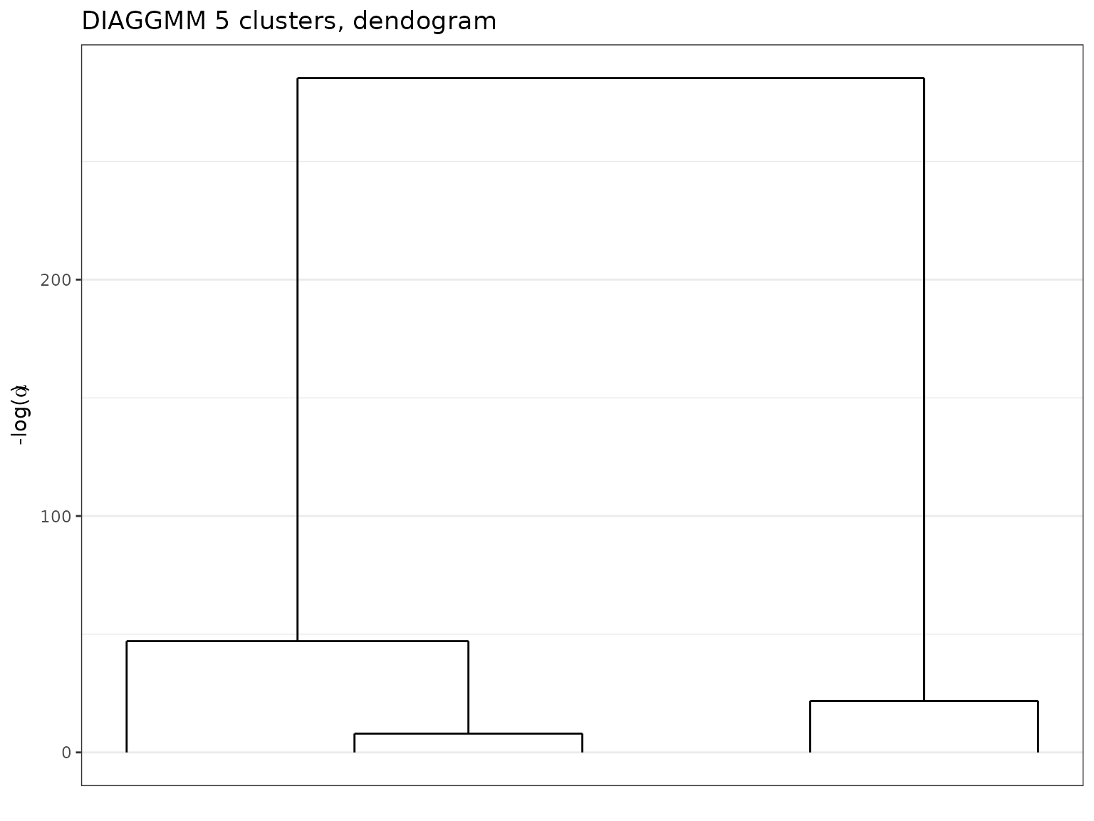

Dendogram extracted with a DiagGmm model on the diabetes data.

Then, one may use the cut() to extract a new clustering at any level of the hierarchy. Here is the solution at \(K=3\):

solK3 = cut(soldiag, K=3)
table(diabetes$cl,clustering(solK3)) %>% knitr::kable()

	1	2	3
Chemical	8	28	0
Normal	71	5	0
Overt	0	3	30

Again, the clusters are relevant compared to the known groups.

Eventually, we may compare the ICL values between the full and diagonal models, using the ICL method and compute their difference to get a quantity similar to Bayes factor with the difference that the partition was not marginalized out, but optimized.

cat('Full GMM has an ICL = ', ICL(sol), '.\n')
#> Full GMM has an ICL =  -263.9857 .
cat('Diagonal GMM has an ICL = ', ICL(soldiag), '.\n')
#> Diagonal GMM has an ICL =  -278.884 .
bayesfactor = ICL(sol)-ICL(soldiag)
cat('Bayes factor = ', bayesfactor, '.\n')
#> Bayes factor =  14.89828 .

The full model achieved a quite better fit on this dataset.

Note: A note on caution on these statistics which take into account the chosen hyperparmaters and may therefore be influenced by the chosen values, as a classical bayes factor. These value must therefore be chosen with care and eventually their impact investigated with a sensibility analysis.

High-dimensional example : the fashion MNIST dataset

As explained above, diagonal models are attractive when working in high-dimensional settings. Their interest is twofold. First, the number of free parameters in the generative model is reduced, which is useful to reduce computational time even though they are integrated out in the ICL. Second, the prior maybe defined such that it will be less informative. We illustrate this with a subset of the fashion-mnist data provided with the package which contains \(p=784\) dimensional vectors (corresponding to 28x28 flattened images of clothing). In this setting, the optimization algorithm is switched to ?`seed-class`, which, while a bit less efficient than the hybrid algorithm used by default in greed(), has a lowest computational burden since it relies on a single and carefully chosen seeded initialization. In addition, we also increase the initial value for \(K\) in order to compensate for the seed method’s inability to find a value of \(K\) bigger than its initialization.

data("fashion")
dim(fashion)
#> [1] 1000  784
sol_fashion=greed(fashion,model=DiagGmm(),alg=Seed(),K=60)
#> 
#> ── Fitting a DIAGGMM model ──
#> 
#> ── Final clustering ──
#> 
#> ── Clustering with a DIAGGMM model 21 clusters and an ICL of -3590254

On this more complex dataset, the clustering found by the algorithm has 21 clusters and the dendrogram proves very informative, highlighting the complex structure of these data.

plot(sol_fashion,type='tree')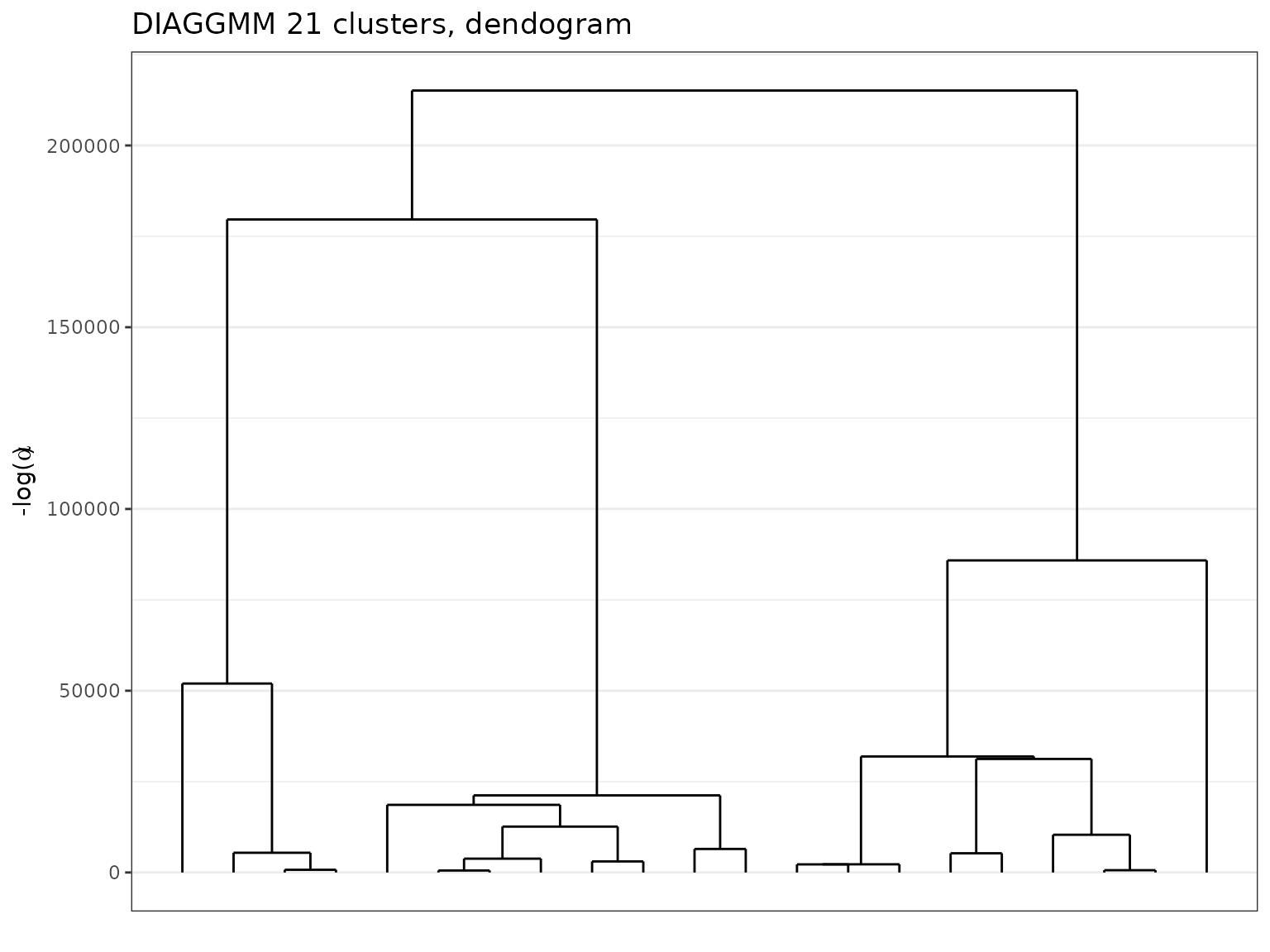

Dendogram extracted with a DiagGmm model on the fashionMNIST data.

Finally, the clusters centers look coherent and the hierarchical ordering underlines a form of “geometric proximities” between cluster objects.

plot_clust_centers <- function(sol) {
  clust_centers = coef(sol)$muk
  im_list=lapply(1:sol@K,function(k){
      data.frame(i=rep(28:1,each=28),j=rep(1:28,28),v=t(clust_centers[[k]]),k=k)
      })
  
  ims = do.call(rbind,im_list)
  gg = ggplot(ims)+
      geom_tile(aes(y=i,x=j,fill=v))+
      scale_fill_gradientn(colors=c("#ffffff","#000000"),guide="none")+
      scale_x_continuous(breaks=c())+scale_y_continuous(breaks=c())+facet_wrap(~k)+
      coord_equal()+theme_minimal()+
      theme(axis.title.x = element_blank(),axis.title.y = element_blank())
  return(gg)
} 
plot_clust_centers(sol_fashion)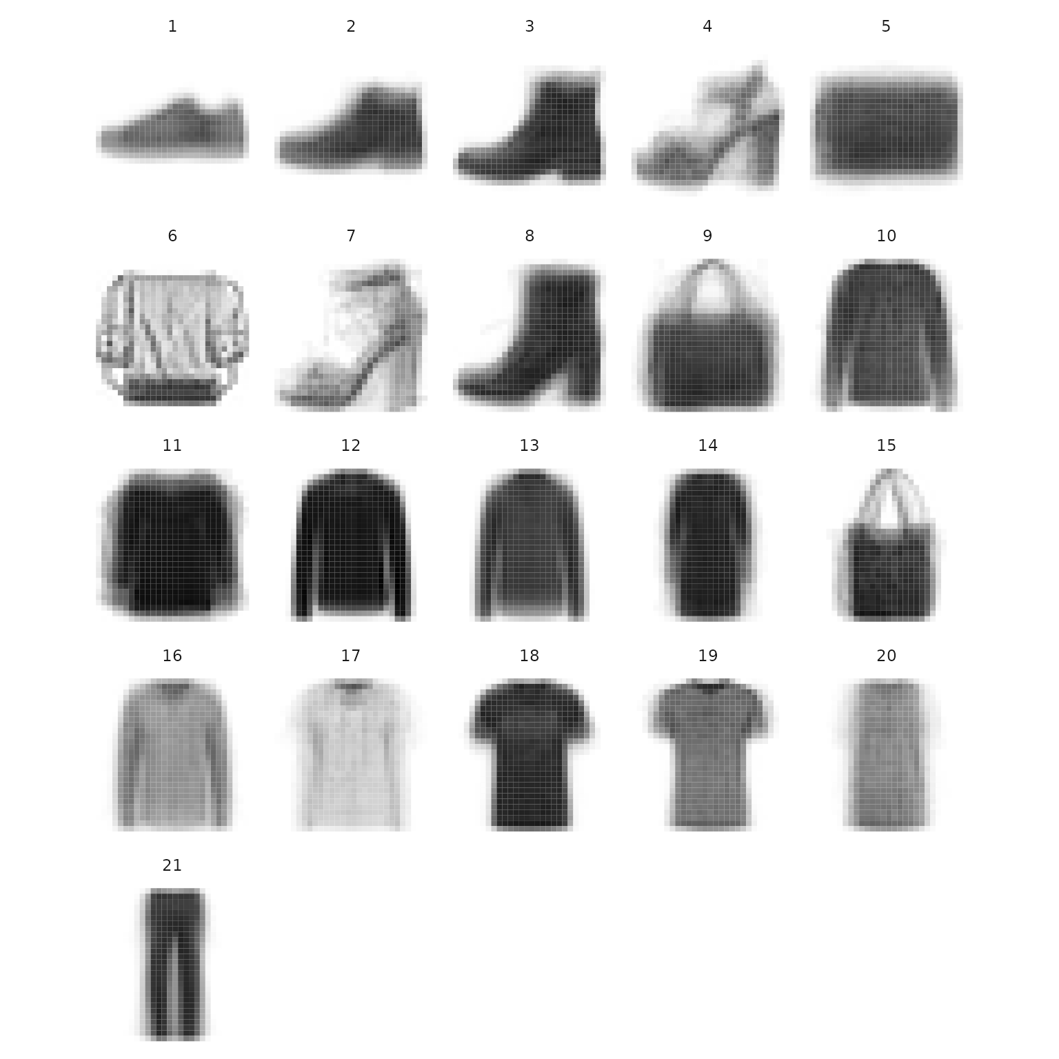

Visualization of the clusters centers extracted on the FashionMNIST data.

As already demonstrated, the clustering can be cut at a coarser levels, if one wants a more synthetic result. We may for example look at the centers for the \(7\)-components clustering:

sol_fashion_K7 = cut(sol_fashion, K=7)
plot_clust_centers(sol_fashion_K7)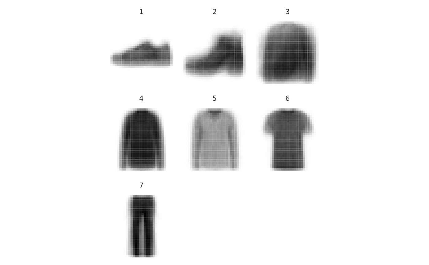

Visualization of the clusters centers extracted on the FashionMNIST data at a coarser level.