Graph clustering with the Stochastic block model
Etienne Côme & Nicolas Jouvin
Source:vignettes/SBM.Rmd
SBM.RmdLoads packages and set a future plan for parallel processing.
library(future) # allows parralel processing in greed()
library(Matrix) # sparse matrix
library(ggplot2) # ploting and data
library(greed)
library(dplyr)
library(ggpubr)
set.seed(2134)

future::plan("multisession", workers=5) # may be increased
The model
Graph data arise in various scientific fields from biology to sociology, and accounts for relationship between objects. These objects are expressed as nodes, while a relationship between two objects is expressed as an edge. Hence, graph data may be expressed and stored in an adjacency matrix \(\mathbf{X} = \{ x_{ij} \}\) where \(x_{ij}=1\) means that objects \(i\) and \(j\) are connected. Weighted versions are also possible.
The stochastic block model (SBM) is a random graph model of the adjacency matrix \(\mathbf{X}\) widely used for graph clustering. In this model, the probability of an edge \((i,j)\) is driven by the cluster membership of node \(i\) and \(j\), hence the block terminology.
It can be expressed in the DLVMs framework and the greed package handles this model and its degree-corrected variant, while implementing efficient visualization tools for the clustering results that we detail below. The Bayesian formulation of a binary SBM is as follows
\[\begin{equation} \label{eq:sbm} \begin{aligned} \pi&\sim \textrm{Dirichlet}_K(\alpha),\\ \theta_{k,l} & \sim \textrm{Beta}(a_0, b_0), \\ Z_i&\sim \mathcal{M}(1,\pi),\\ \forall (i,j), \quad x_{ij} \mid Z_{ik}Z_{jl}=1& \sim \mathcal{B}(\theta_{k,l}). \end{aligned} \end{equation}\]This model class is implemented in the ?Sbm class. Here,
the model hyperparameters are:
- \(\alpha\) which is set to \(1\) by default.
- The beta distribution parameters \(a_0\) and \(b_0\) on the connectivity matrix \(\mathbf{\theta}\). A non-informative prior
can be chose with \(a_0=b_0=1\), which
is the default value in
Sbm.
Note that the greed package also handles the degree-corrected variant
of SBM in the ?dcSbm class, allowing for integer valued
edges. The underlying model and its DLVM formulation is described in
depth in the Supplementary Materials of Côme et.
al..
An introductory example: SBM with hierarchical structure
Simulation scenario
We begin by simulating from a hierarchically structured SBM model,
with 2 large clusters, each composed of 3 smaller clusters with higher
connection probabilities, making a total of 6 clusters. Greed comes
shipped with simulation function for the different generative models it
handle and we will take advantage of the `rsbm() function
to simulate an SBM graph with 6 clusters and 400 nodes:
N  <- 400           # Number of node
K  <- 6             # Number of cluster
pi <- rep(1/K,K)    # Clusters proportions
lambda   <- 0.1     # Building the connectivity matrix template
lambda_o <- 0.01
Ks <- 3
mu <- bdiag(lapply(1:(K/Ks), function(k){
  matrix(lambda_o,Ks,Ks)+diag(rep(lambda,Ks))}))+0.001
sbm <- rsbm(N,pi,mu) # Simulation
The connectivity pattern used for the simulation, present a small hierarchical structure with two big clusters each composed of three sub clusters with a community like pattern:
| 0.111 | 0.011 | 0.011 | 0.001 | 0.001 | 0.001 |
| 0.011 | 0.111 | 0.011 | 0.001 | 0.001 | 0.001 |
| 0.011 | 0.011 | 0.111 | 0.001 | 0.001 | 0.001 |
| 0.001 | 0.001 | 0.001 | 0.111 | 0.011 | 0.011 |
| 0.001 | 0.001 | 0.001 | 0.011 | 0.111 | 0.011 |
| 0.001 | 0.001 | 0.001 | 0.011 | 0.011 | 0.111 |
Clustering with the greed() function
As always, we perform the clustering using the greed()
function with an Sbm model. Note that we need to specify
the Sbm model, since for squared sparse matrix the default
model used is a DcSbm. By default, the hybrid genetic
algorithm is used, and its default hyperparameters are detailed in
?`Hybrid-class`.
class(sbm$x)
#> [1] "dgCMatrix"
#> attr(,"package")
#> [1] "Matrix"
sol <- greed(sbm$x,model = Sbm())
#>
#> ── Fitting a guess SBM model ──
#>
#> ℹ Initializing a population of 20 solutions.
#> ℹ Generation 1 : best solution with an ICL of -14632 and 13 clusters.
#> ℹ Generation 2 : best solution with an ICL of -14214 and 8 clusters.
#> ℹ Generation 3 : best solution with an ICL of -14119 and 6 clusters.
#> ℹ Generation 4 : best solution with an ICL of -14119 and 6 clusters.
#> ── Final clustering ──
#>
#> ── Clustering with a SBM model 6 clusters and an ICL of -14119
We see that the fine-grained clustering structure with \(K=6\) clusters is recovered.
Note: For network data, and Sbm like models, greed accept an adjacency matrix of class
Matrix::dgCMatrixlike in the previous example, but the network can also be provided as a simplematrixor as anigraphobject.
Inspecting the clustering results
The result of greed is stored as an S4 class and, as for
any model, there are dedicated function to access its attributed. A
quick summary of these functions is indicated in the display of the
sol object as follows
sol
#>
#> ── Clustering with a SBM model 6 clusters and an ICL of -14119 ──
#>
#> ℹ Generic methods to explore a fit:
#> • ?clustering, ?K, ?ICL, ?prior, ?plot, ?cut, ?coef
The clustering() function allows to return the estimated
partition. The K() and ICL() functions return
the final number of clusters and ICL value respectively.
table(sbm$cl,clustering(sol))| 1 | 2 | 3 | 4 | 5 | 6 | |
|---|---|---|---|---|---|---|
| 1 | 0 | 63 | 0 | 0 | 0 | 0 |
| 2 | 0 | 0 | 66 | 0 | 0 | 0 |
| 3 | 64 | 0 | 0 | 0 | 0 | 0 |
| 4 | 0 | 0 | 0 | 0 | 0 | 79 |
| 5 | 0 | 0 | 0 | 60 | 0 | 0 |
| 6 | 0 | 0 | 0 | 0 | 68 | 0 |
The Maximum a Posteriori (MAP) estimation of \(\theta\) and \(\pi\) is available through the
coef() function. Note that the MAP is computed
conditionally to the estimated partition returned by
greed.
| 0.119 | 0.011 | 0.010 | 0.001 | 0.001 | 0.001 |
| 0.013 | 0.113 | 0.009 | 0.000 | 0.000 | 0.001 |
| 0.012 | 0.010 | 0.109 | 0.002 | 0.001 | 0.000 |
| 0.001 | 0.001 | 0.002 | 0.114 | 0.008 | 0.011 |
| 0.001 | 0.001 | 0.001 | 0.014 | 0.115 | 0.011 |
| 0.001 | 0.001 | 0.001 | 0.010 | 0.011 | 0.105 |
We may observe, as expected, that the MAP estimate of the connectivity pattern is close to the one used for the simulation.
Visualization tools
The greed package also comes with efficient visualization tools for summarization and exploration. For graph data, it allows to:
- Plot the aggregated adjacency matrix between the estimated clusters, with colors indicating link density.
- Plot a node-link diagram representation of the clustering, where each cluster is represented as a point and arrow width indicates link density.
- Plot the dendrogram extracted via the hierarchical clustering
algorithm from
K(sol)to1with the required level of regularization \(\log(\alpha)\).
Note that, in each case, the ordering of the clusters given by the hierarchical algorithm is used and greatly enhances the visualization by highlighting the hierarchical structure in the data.
Block representation of the adjacency matrix
plot(sol,type='blocks')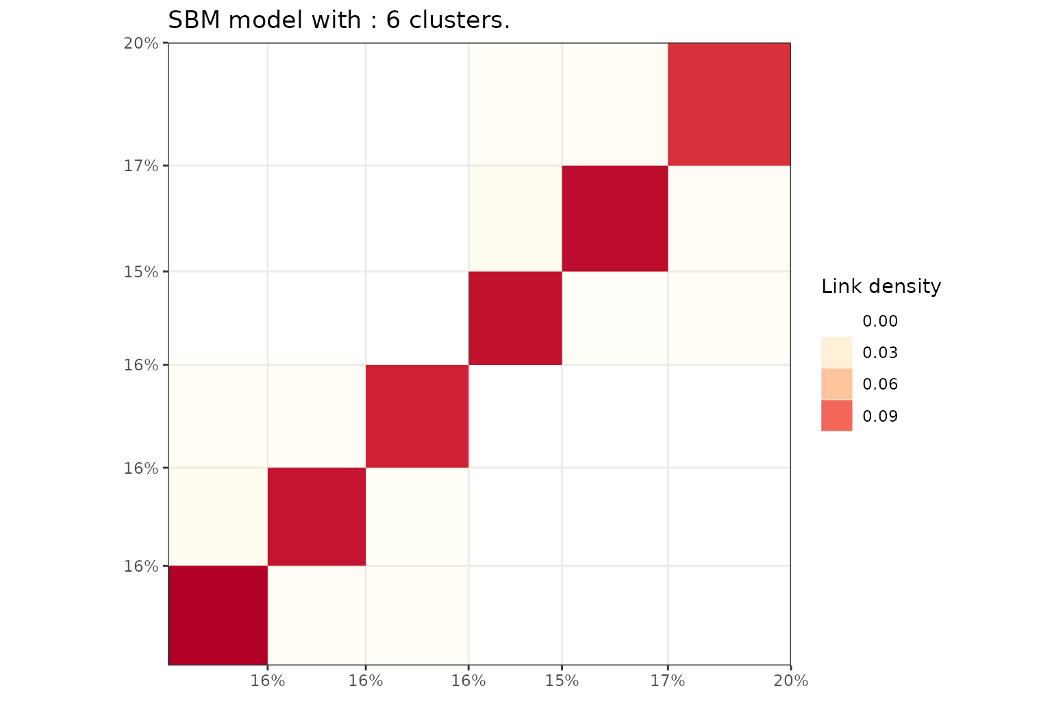
Block representation of the SBM results.
Node link diagram of the clustering result
plot(sol,type='nodelink')
Cluster and link representation of the SBM results.
Dendrogram representation of the hierarchical clustering
plot(sol,type='tree')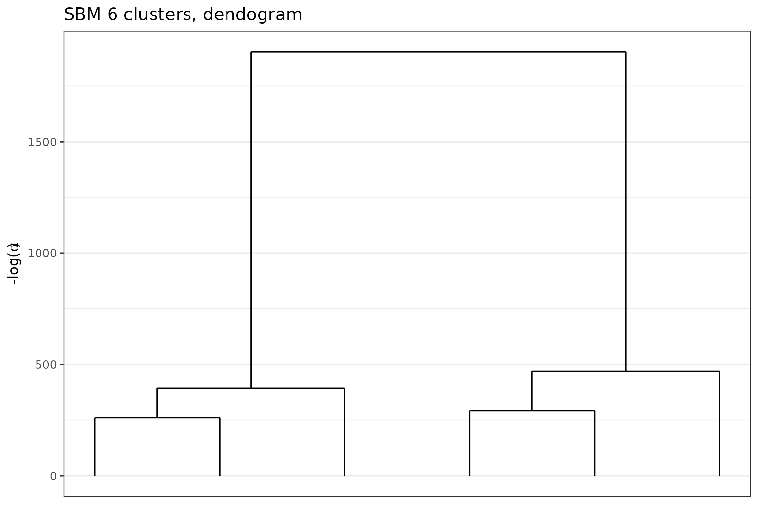
Dendogram representation of the greed result on the simulated Sbm data.
Exploring the hierarchy
Eventually, we can cut the dendrogram at any level below
K(sol) to easily access other partitions in the hierarchy.
Here, we access the coarser at \(K=2\)
and we can still use the different plot() functions to
visualize these other solutions.
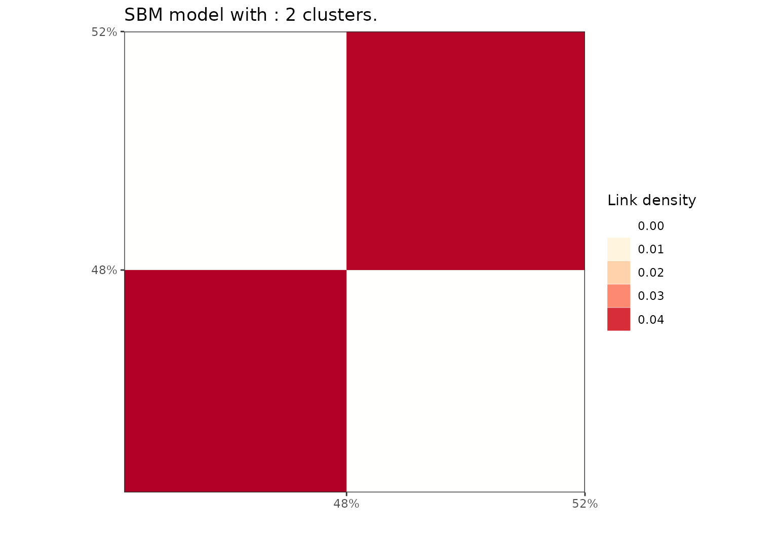
Block representation of the SBM results after cutting at K=2.
Choosing the cut level
Choosing relevant level(s) to cut the dendrogram may be
challenging and the greed package also provides
graphical tools to help the user decide based on a chosen
heuristics.
- One can search for changepoints in the evolution of \(-log(\alpha)\) with respect to \(K\) with the following plot:
plot(sol,type='path')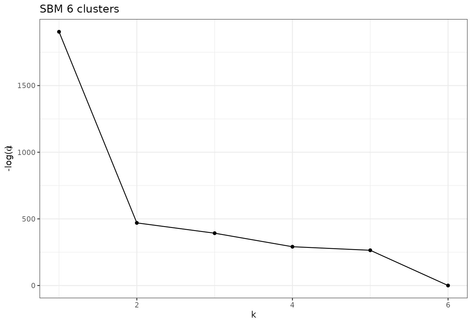
Path plot, evolution of regularization with respect to \(K\)
- Or of the ICL value with respect to \(log(\alpha)\), with the Pareto front highlight the range of dominance of each partition in the hierarchy.
plot(sol,type='front')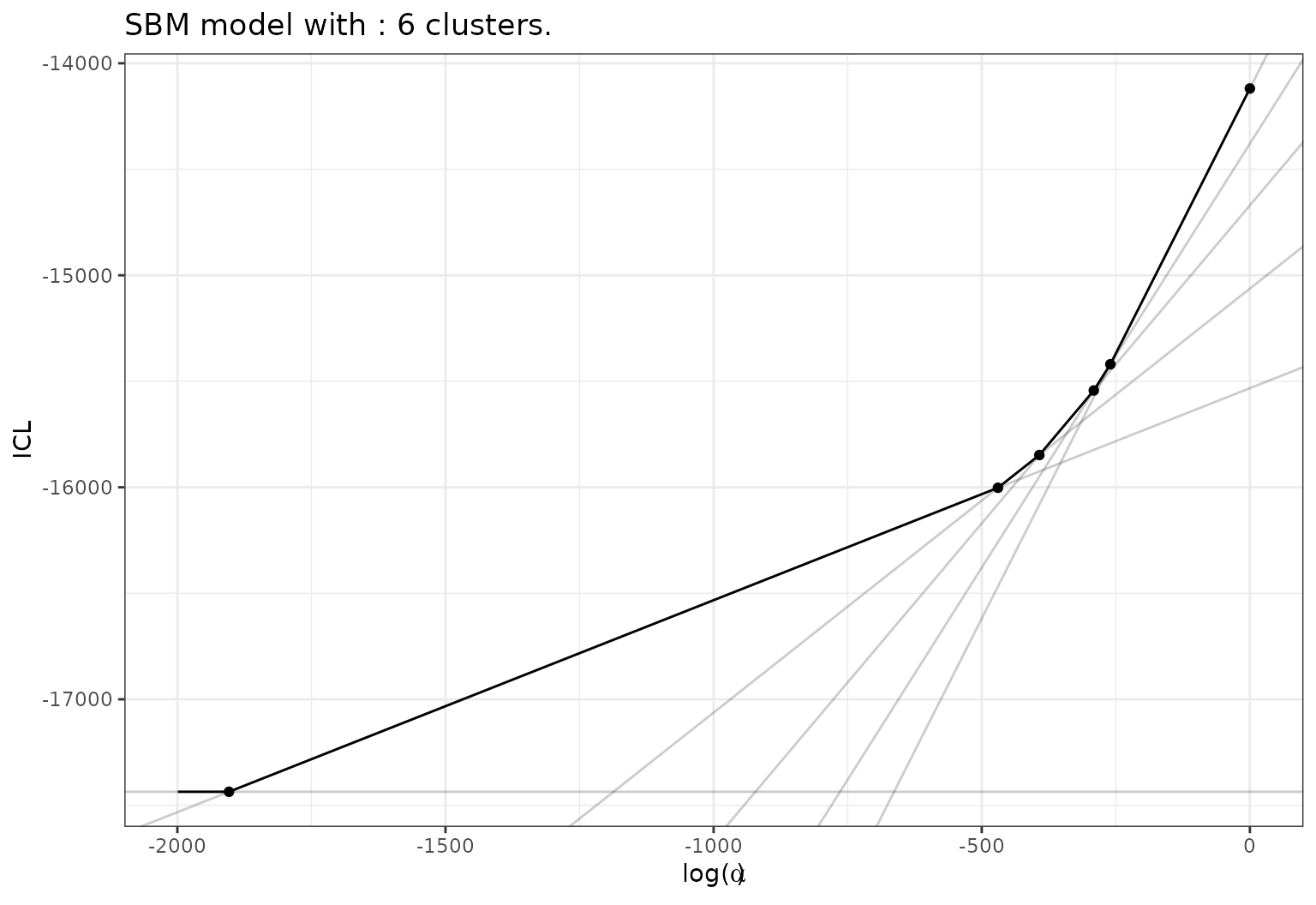
Degree corrected variant
Here, we compare models with and without degree correction on DcSbm
simulation (see ?rdcsbm).
sim_dcsbm <- rdcsbm(N,pi,mu,round(rexp(N,1/15)),round(rexp(N,1/15)))
X <- sim_dcsbm$x
X[X>1] <- 1 # Sbm model may only deal with binary adjacency matrix
sol_dcsbm <- greed(X,model = DcSbm()) # DcSbm model allow for weighted graph with counts for the weights
#>
#> ── Fitting a guess DCSBM model ──
#>
#> ℹ Initializing a population of 20 solutions.
#> ℹ Generation 1 : best solution with an ICL of -11620 and 7 clusters.
#> ℹ Generation 2 : best solution with an ICL of -11553 and 6 clusters.
#> ℹ Generation 3 : best solution with an ICL of -11553 and 6 clusters.
#> ── Final clustering ──
#>
#> ── Clustering with a DCSBM model 6 clusters and an ICL of -11553
sol_sbm <- greed(X,model = Sbm())
#>
#> ── Fitting a guess SBM model ──
#>
#> ℹ Initializing a population of 20 solutions.
#> ℹ Generation 1 : best solution with an ICL of -12975 and 12 clusters.
#> ℹ Generation 2 : best solution with an ICL of -12726 and 13 clusters.
#> ℹ Generation 3 : best solution with an ICL of -12619 and 12 clusters.
#> ℹ Generation 4 : best solution with an ICL of -12567 and 12 clusters.
#> ℹ Generation 5 : best solution with an ICL of -12548 and 12 clusters.
#> ℹ Generation 6 : best solution with an ICL of -12538 and 12 clusters.
#> ℹ Generation 7 : best solution with an ICL of -12534 and 11 clusters.
#> ℹ Generation 8 : best solution with an ICL of -12531 and 12 clusters.
#> ℹ Generation 9 : best solution with an ICL of -12531 and 12 clusters.
#> ── Final clustering ──
#>
#> ── Clustering with a SBM model 11 clusters and an ICL of -12525
As expected the degree corrected version did a better job as the ICL value suggest. Indeed, without degree correction, the model has to use more groups to fit the degree heterogeneity.
A real data example: the Books dataset
The Books dataset was gathered by Valdis Krebs and is attached to the greed package. It consist of a co-purchasing network of \(N=105\) books on US politics. Two books have an edge between them if they have been frequently co-purchased together. We have access to the labels of each book according to its political inclination: conservative (“n”), liberal (“l”) or neutral (“n”).
data(Books)

sol_dcsbm <- greed(Books$X,model = DcSbm())
#>
#> ── Fitting a guess DCSBM model ──
#>
#> ℹ Initializing a population of 20 solutions.
#> ℹ Generation 1 : best solution with an ICL of -1350 and 4 clusters.
#> ℹ Generation 2 : best solution with an ICL of -1346 and 4 clusters.
#> ℹ Generation 3 : best solution with an ICL of -1346 and 4 clusters.
#> ── Final clustering ──
#>
#> ── Clustering with a DCSBM model 3 clusters and an ICL of -1345

sol_sbm   <- greed(Books$X,model = Sbm())
#>
#> ── Fitting a guess SBM model ──
#>
#> ℹ Initializing a population of 20 solutions.
#> ℹ Generation 1 : best solution with an ICL of -1259 and 5 clusters.
#> ℹ Generation 2 : best solution with an ICL of -1251 and 6 clusters.
#> ℹ Generation 3 : best solution with an ICL of -1251 and 6 clusters.
#> ── Final clustering ──
#>
#> ── Clustering with a SBM model 5 clusters and an ICL of -1249
The network as been automatically recognized as an undirected graph, as we can see see in the fitted models prior:
For this dataset, the regular SBM model seems to reach a better ICL solution than its degree-correction variant. Still, we can visualize both aggregated adjacency matrices and the dendrogram.
bl_sbm = plot(sol_sbm,type='blocks')
bl_dcsbm = plot(sol_dcsbm,type='blocks')
ggarrange(bl_sbm,bl_dcsbm)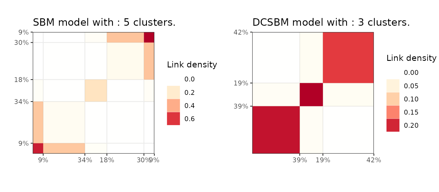
Block matrix representation of the DcSbm and Sbm solution found with greed on the Book network.
It is also possible to use external R packages to plot the graph layout with node color as clusters and node size as book popularity (computed using centrality degree). Here, we represent the result for the SBM solution with 5 clusters. One can see a hierarchical clustering structure appearing, with a central cluster of neutral books in-between two densely connected set. In each of these two dense set, there is a clear distinction between popular books (heavily purchase) and more peripheral ones, indicated by node size.
library(ggraph)
library(tidygraph)
library(igraph)

graph <- igraph::graph_from_adjacency_matrix(Books$X) %>% as_tbl_graph() %>%
    mutate(Popularity = centrality_degree())  %>%
    activate(nodes) %>%
    mutate(cluster=factor(clustering(sol_sbm),1:K(sol_sbm)))

# plot using ggraph
ggraph(graph, layout = 'kk') +
    geom_edge_link() +
    geom_node_point(aes(size = Popularity,color=cluster))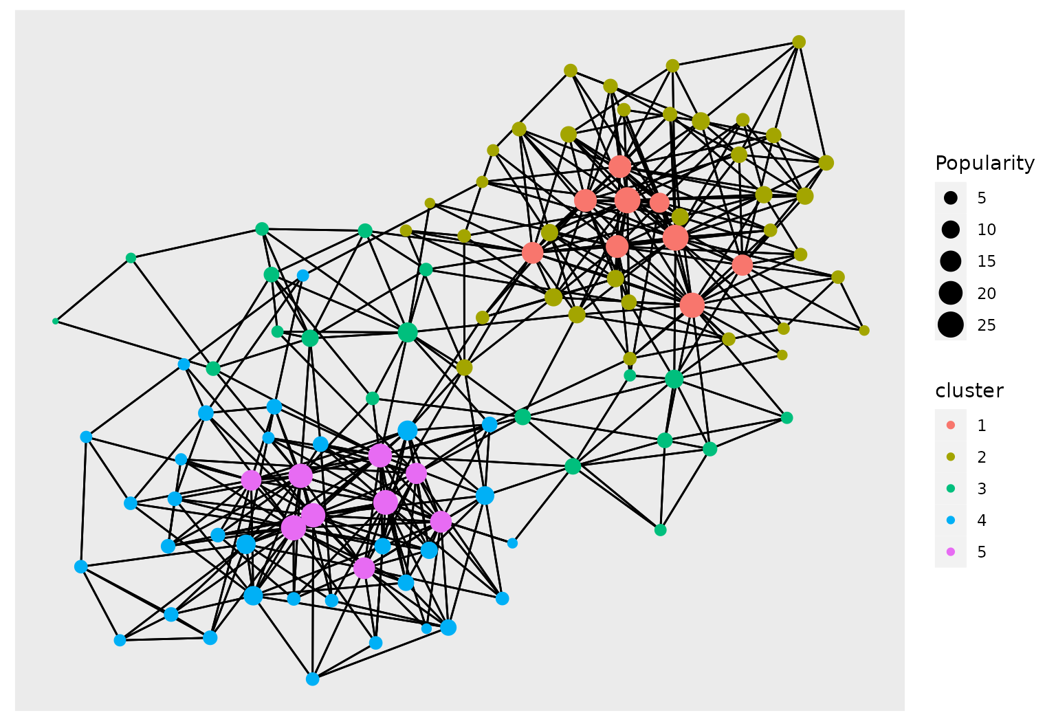
Ggraph plot of the book network with node colors given by the clustering found with greed and an Sbm model.
Finally, we can look at both models solutions for \(K=3\) and their confusion matrix. We see that both partition make sense according to the available political label.
|
|
Categorical edges and multidimensional networks
Sometimes, a graph accounts for more complex interactions between object such as:
- categorical relationship instead of solely binary
- multidimensional/multilayered relationships encoded by different graphs (e.g. work relation and friendship)
The first case can be addressed in the SBM framework via a
multinomial SBM model. The second is different since there are different
layer or views of the data. Still, the greed
package may handle this type of data via its CombinedModels
framework where user simply stacks the DLVM of its choice on each view
of the data (for more info see the dedicated vignette on Combined
Models).
Categorical edges and the Multinomial SBM: newguinea dataset
The SBM framework allows virtually any distribution on the edges,
hence allowing to handle categorical edges modeled as multinomial random
variables. With the right choice of conjugate Dirichlet priors, this
model admits an exact ICL formulation which allows to use the
greed framework. This model is implemented in the
MultSbm S4 class and we illustrate its use on a toy data
set consisting in interactions between \(n=16\) tribes. This interaction can be one
of 3 types: enemies, friends or no relation. These are encoded as 3
dimensional one-hot vectors in the NewGuinea dataset.
sol_newguinea = greed(NewGuinea,model=MultSbm())
#>
#> ── Fitting a guess MULTSBM model ──
#>
#> ℹ Initializing a population of 20 solutions.
#> ℹ Generation 1 : best solution with an ICL of -127 and 3 clusters.
#> ℹ Generation 2 : best solution with an ICL of -127 and 3 clusters.
#> ── Final clustering ──
#>
#> ── Clustering with a MULTSBM model 2 clusters and an ICL of -123
Practicalities: The
MultSbmmodel allows only input in the form of anarrayobject with dimensions N,N,M with N the number of nodes and M the number of modalities. Such representation is not sparse and therefore, this type of model will not scale well with N.
To each modality (or slice), we can associate a binary graph corresponding to the interaction, and plot its aggregated adjacency matrix. The multiple views allow to interpret the clusters in term of the modalities. In this example, we have three slices corresponding to the three modalities and :
- In the first modality (enmity), group 1 and 2 have more interaction outside than within the groups (enemies fight more than friends)
- The second slice (friendship) is consistent with the first slice, since the two groups have a pronounced community structure, with group 2 being small and densely connected. There are no friendships links between the two groups.
- The third slice (no relation) highlight that individuals in group 1 mostly share less relations.
To sum up, the algorithm found \(K=2\) groups/clusters. One is composed of a small, densely connected community of friend tribes, whereas the other is larger and more heterogeneous with less interactions between the tribes. The two clusters either have enmity relations or no relation at all.
plot(sol_newguinea,type='blocks')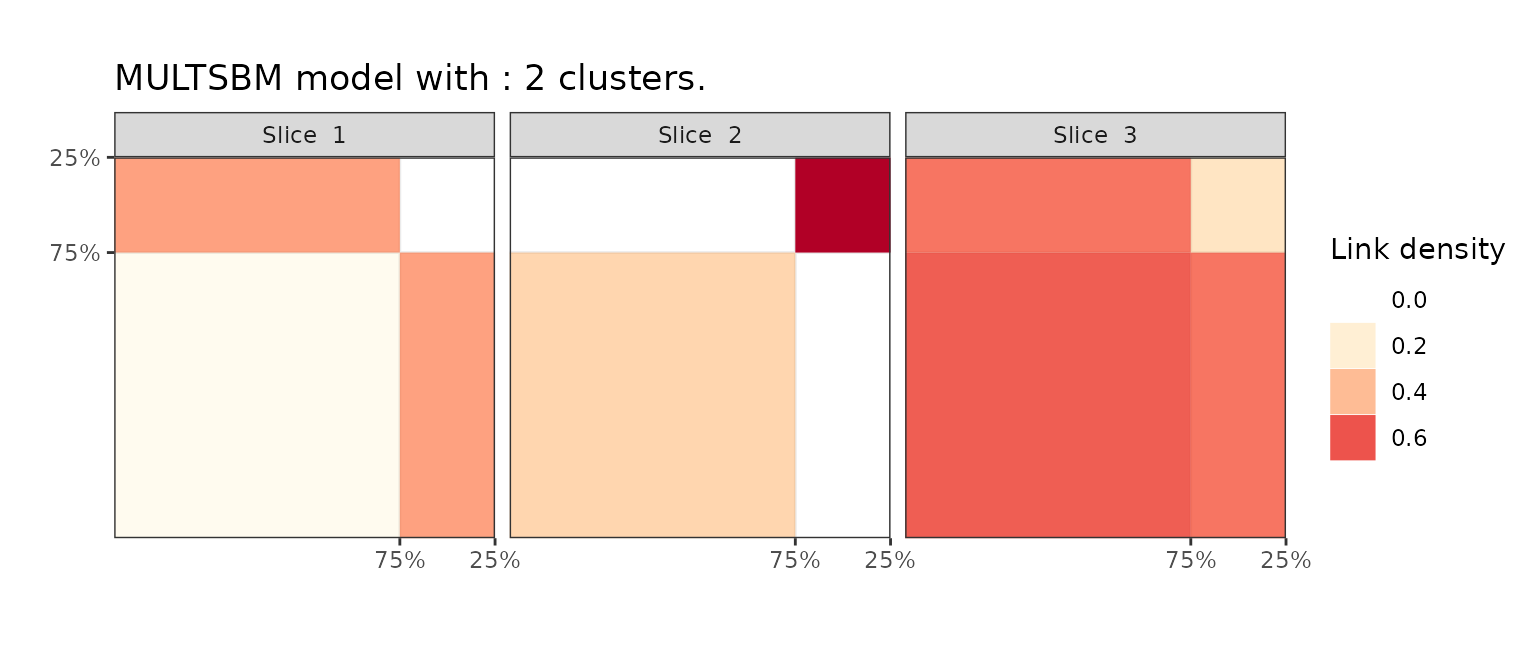
Block matrix plot of the MultSbm results on the NewGuinea network.
To further the analysis, it is possible to visualize the two graphs of enmity and friendships on top of each other. The node shape symbolizes the cluster, while the color of the edge characterizes the modality. One can see that the small cluster makes a 4-node clique for friendship while having a strongly pronounced bi-partite structure for enmity, hence consistent with the previous analysis.
enemies = as.data.frame(which(NewGuinea[,,1]==1,arr.ind = TRUE)) %>%
  mutate(relation="enemy")
friends = as.data.frame(which(NewGuinea[,,2]==1,arr.ind = TRUE)) %>%
  mutate(relation="friend")

edges = rbind(enemies,friends)
graph = tbl_graph(edges=edges,nodes=data.frame(id=1:16,cluster=factor(clustering(sol_newguinea))))

# plot using ggraph
ggraph(graph, layout = 'kk', weights = if_else(relation=="friends",1,0)) +
    geom_edge_link(aes(color=relation),width=1.2) +
    scale_edge_color_manual(values = c("friend"="#4398cc","enemy"="#b60000"))+
    geom_node_point(aes(shape=cluster),size=5)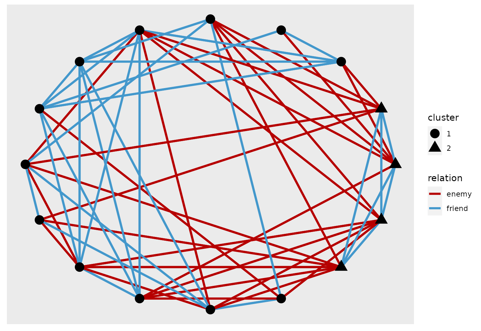
Ggraph plot of the NewGuinea network with the result of the MultSbm model.
General case: multidimensional networks and mixed-models
As explained above, some graphs may encode different kinds of relationships. This general case of multidimensional network correspond to a 3-dimensional encoding \(V\) different graphs. Note that graphs with multinomial edges are a particular case where an edge \((i,j)\) can only belong to one of the views.
In the perspective of graphs clustering, we search for one common partition of the nodes among the different graphs. From the statistical point-of-view of the DLVMs framework, it amounts to stack observational models (i.e. SBM, dc-SBM, MultinomialSBM, etc.) on each of the graphs, that are supposed independent conditionally on the unknown partitions :
\[\begin{equation} p(G_1, \ldots, G_V \mid Z) = p(G_1 \mid Z) \times \ldots \times p(G_V \mid Z). \end{equation}\]The ICL of the whole dataset is then simply the sum of the individual ICL of the V models.
The greed package implements this modelisation via
the ?CombinedModels-class. We refer to the dedicated
vignettes for more details vignette("Mxixed-Models") but,
from a practical perspective, one need to specify the \(V\) observational models in a named list,
and the data (here the \(V\) adjacency
matrices) in a list sharing the same names. Here is an example on the
NewGuinea dataset analyzed above, with \(V=2\) views corresponding to enmity and
friendship. We put a default DcSBM model on both views and provide the
two corresponding adjacency matrix as data.
mod <- CombinedModels(list(friends = DcSbmPrior(), enmy = DcSbmPrior()))
data <- list(friends = NewGuinea[, , 2], enmy = NewGuinea[, , 1])
sol_bidcsbm <- greed(data, model = mod, K = 5)
#>
#> ── Fitting a COMBINEDMODELS model ──
#>
#> ℹ Initializing a population of 20 solutions.
#> ℹ Generation 1 : best solution with an ICL of -151 and 2 clusters.
#> ℹ Generation 2 : best solution with an ICL of -151 and 2 clusters.
#> ── Final clustering ──
#>
#> ── Clustering with a COMBINEDMODELS model 2 clusters and an ICL of -151
Practicalities: The
CombinedModelsclass allows any list of observational models. However, they need to be initiated via the following syntax:<your_desired_model>Prior(). Without going into technical details, this is necessary to account for the shared aspect of the partition \(Z\) between all models.
Practicalities: A
CombinedModelswithSbmPriororDcSbmPriorviews will use a sparse representation of the different views and will therefore scale well with the network size.
The algorithm finds \(K=2\) clusters
here. Since each views has its own observational model, it is possible
to use the ?extractSubModel() function to retrieve the
fitted observational model for each view. Then, traditional
visualization tools may be used. Here, we display the block
representation of the clustering for the two modalities, highlighting a
pronounced community structure in the friendship modality and a
strong bipartite structure in the enmity modality as before,
with no enmity link in the small cluster and few among the tribes of the
bigger one.
bl_friends <- plot(extractSubModel(sol_bidcsbm,"friends"),type="blocks") + ggtitle("Friendship")
bl_enmy <- plot(extractSubModel(sol_bidcsbm,"enmy"),type="blocks") + ggtitle("Enmity")
ggarrange(bl_friends,bl_enmy)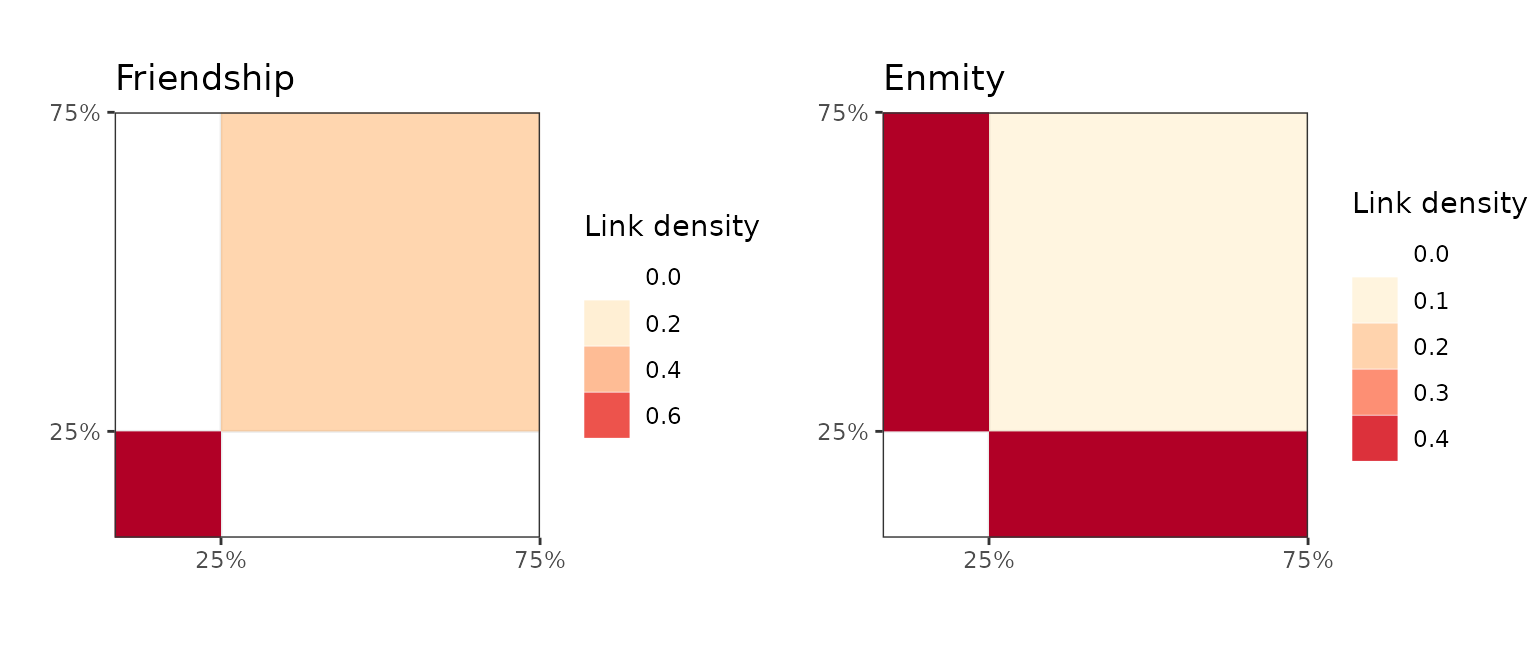
Block matrix repressentation of the clustering with the two views.
7th grade dataset
The ?SevenGraders dataset illustrates the interest of
multidimensional graphs clustering. There are 3 different relationship
(class, best-friends and work) recorded between 29 seventh-grade
students in Victoria, Australia. We also have access to the gender of
each student: 1 to 12 are boys and 13 to 29 are girls.
We are interested in finding an underlying partition explaining these
\(3\) kinds of relationships. Again, we
put a DcSbmPrior model for each view, and provide the
models and views as named lists with the same names.
mod <- CombinedModels(list(class = DcSbmPrior(), friends = DcSbmPrior(), work = DcSbmPrior()))
data <- list(class = SevenGraders[, , 1], friends = SevenGraders[, , 2], work = SevenGraders[, , 3])
sol <- greed(data, model = mod, K = 5)
#>
#> ── Fitting a COMBINEDMODELS model ──
#>
#> ℹ Initializing a population of 20 solutions.
#> ℹ Generation 1 : best solution with an ICL of -1519 and 4 clusters.
#> ℹ Generation 2 : best solution with an ICL of -1514 and 4 clusters.
#> ℹ Generation 3 : best solution with an ICL of -1514 and 4 clusters.
#> ── Final clustering ──
#>
#> ── Clustering with a COMBINEDMODELS model 4 clusters and an ICL of -1514
Here, the algorithm found \(K=4\) clusters and we can look at the block matrix representation of the work relation graph.
plot(extractSubModel(sol, "work"), type = "blocks")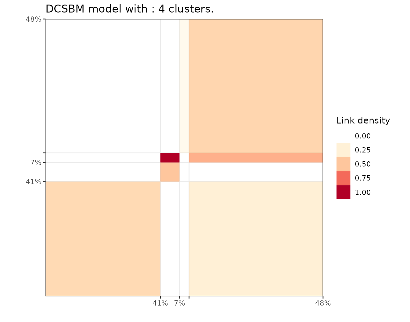
Block matrix representation of the work layer clustering found with multi DcSbm clustering.