Loads packages.
library(future) # allows parralel processing in greed()
library(greed)
library(mclust)
library(ggplot2)
library(ggsoccer)
library(dplyr)
library(tidyr)
set.seed(2134)

future::plan("multisession", workers=2) # may be increased
Mixture of Regression
Mixture of Regressions as their name suggest fit several regression models at the same time and try to extract a partition where different regression models holds for each subsets. Formally, the Bayesian version of this model with invariant priors is given by the following generative model.
\[ \begin{align} \pi &\sim Dirichlet(\alpha)\\ Z_i &\sim \mathcal{M}(1,\pi)\\ V_k &\sim \mathcal{W}(\varepsilon^{-1},n_0)\\ A_k|V_k,X &\sim \mathcal{MN}(0,(V_k)^{-1},\tau X^{t}X)\\ Y_{i.}|X_{i.},Z_{ik}=1 &\sim \mathcal{N}(A_kx_{i.},V_{k}^{-1}) \end{align} \] with \(\mathcal{MN}()\) the matrix normal distribution and \(\mathcal{W}()\) the Whishart distribution. The prior parameters may therefore have an impact on the results and they can’t be non-informative. The main prior parameters to look at are \(\tau\) and \(\varepsilon\). \(\tau\) define the strength of the regularization applied on the regression problem, by default it equals \(0.01\), \(\varepsilon\) and \(n_0\) define the prior for the noise co-variance matrix. By default, it will be equal to 0.1 time the variance of the regression residuals with only one cluster and \(n_0\) is fixed by default to \(d\) the dimension of \(y\) for the prior to be as uninformative as possible.
An introductory example
To introduce this model we will use a small toy artificial dataset
from the flexmix package. The dataset correspond to two
groups. One with a linear relationship between \(x\) and \(y\) and a second with a quadratic
relationship between \(x\) and \(y\) :
data("NPreg", package = "flexmix")
ggplot(NPreg)+geom_point(aes(x=x,y=yn,color=factor(class)))+theme_bw()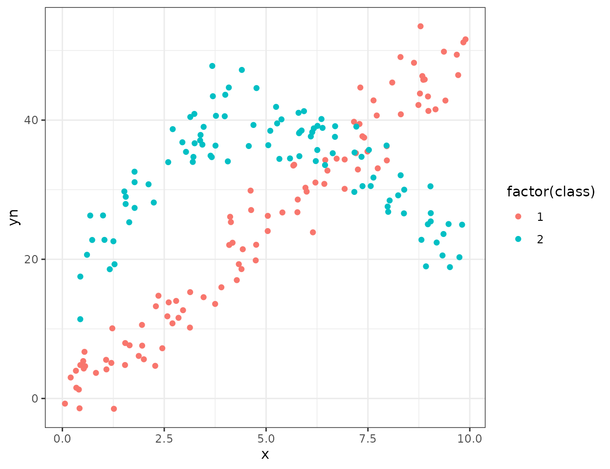 To fit a mixture of regression model with greed, you must provide a
data.frame and a MoR model. To build such a
model, we simply use the MoR function which has one
mandatory argument, the formula of the supposed regression model. In our
toy case, we may thus use the following line of code to fit the
clustering model using a polynomial regression model of degree two:
sol=greed(NPreg,model=MoR(yn ~ x + I(x^2)))
#>
#> ── Fitting a MOR model ──
#>
#> ℹ Initializing a population of 20 solutions.
#> ℹ Generation 1 : best solution with an ICL of -675 and 2 clusters.
#> ℹ Generation 2 : best solution with an ICL of -675 and 2 clusters.
#> ── Final clustering ──
#>
#> ── Clustering with a MOR model 2 clusters and an ICL of -675
As expected the partition with two cluster that was used to simulate
the data is recovered by the algorithm. When, the clustering is
performed, we may use the classical functions
clustering,coef,prior,plot,... to explore the results. We
may start by comparing the found clustering with the true labels :
cl = clustering(sol)
table(cl,NPreg$class)
#>
#> cl   1  2
#>   1  4 95
#>   2 96  5
Look at the value used for the prior parameters :
prior(sol)
#> An object of class "MoR"
#> Slot "formula":
#> yn ~ x + I(x^2)
#>
#> Slot "tau":
#> [1] 0.1
#>
#> Slot "N0":
#> [1] 1
#>
#> Slot "epsilon":
#>          [,1]
#> [1,] 16.88241
#>
#> Slot "alpha":
#> [1] 1
Extract the MAP model coefficient for further use :
params = coef(sol)
params
#> $pi
#>       [,1]
#> [1,] 0.495
#> [2,] 0.505
#>
#> $A
#> $A$cluster1
#>                     yn
#> (Intercept) 13.1690893
#> x            9.0655610
#> I(x^2)      -0.8937771
#>
#> $A$cluster2
#>                      yn
#> (Intercept) -0.33244435
#> x            4.42810766
#> I(x^2)       0.03041496
#>
#>
#> $Sigmak
#> $Sigmak$cluster1
#>         yn
#> yn 11.7112
#>
#> $Sigmak$cluster2
#>          yn
#> yn 11.32306
And plot prediction line of the fitted sub-models:
df.pred = data.frame(x=seq(0,10,length.out=200))
X=model.matrix(~ x +I(x^2),df.pred)
df.mpred = data.frame(sapply(params$A,function(A){X%*%A}))
names(df.mpred)=c("cluster1","cluster2")
df.mpred$x = df.pred$x
ggplot(NPreg)+
  geom_point(aes(x=x,y=yn,color=factor(class)))+
  geom_line(data=df.mpred,aes(x=x,y=cluster1))+
  geom_line(data=df.mpred,aes(x=x,y=cluster2))+
  theme_bw()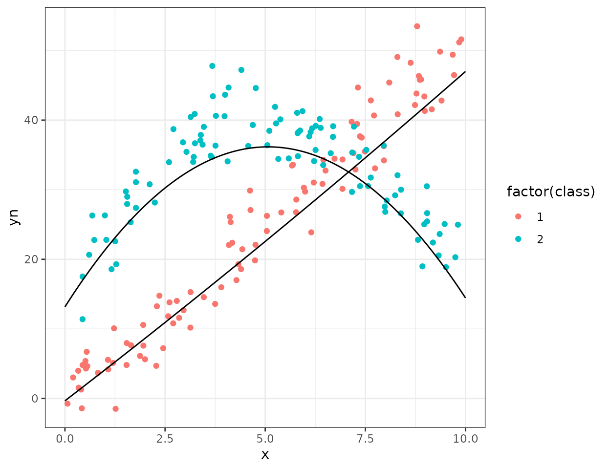
An more challenging application with the Fifa dataset
For this example we will use the Fifa dataset and take a subsample of 2000 players:
data("Fifa")
Xreg=Fifa %>%
    filter(value_eur>0) %>%
  sample_n(2000) %>%
  mutate_if(is.character,as.factor)
We will try to predict the log of the player value from it’s age and ability scores. We therefore define the model and run the clustering in a similar fashion as previously:
reg_formula <- log(value_eur) ~ age + pace + shooting + dribbling + passing + defending  + physic
mod_reg = MoR(reg_formula)
sol=greed(Xreg,mod_reg)
#>
#> ── Fitting a MOR model ──
#>
#> ℹ Initializing a population of 20 solutions.
#> ℹ Generation 1 : best solution with an ICL of -2426 and 2 clusters.
#> ℹ Generation 2 : best solution with an ICL of -2358 and 3 clusters.
#> ℹ Generation 3 : best solution with an ICL of -2344 and 2 clusters.
#> ℹ Generation 4 : best solution with an ICL of -2344 and 2 clusters.
#> ── Final clustering ──
#>
#> ── Clustering with a MOR model 2 clusters and an ICL of -2344
The clustering found has two clusters, if we look at the regression models parameters :
cl=clustering(sol)
co=coef(sol)
co$A
#> $cluster1
#>                value_eur
#> (Intercept)  1.777047269
#> age         -0.081247196
#> pace         0.003948173
#> shooting     0.001935624
#> dribbling    0.015872369
#> passing      0.005951686
#> defending    0.143965128
#> physic       0.027494091
#>
#> $cluster2
#>                value_eur
#> (Intercept)  2.591431380
#> age         -0.066321679
#> pace        -0.001049727
#> shooting     0.034219699
#> dribbling    0.102232855
#> passing      0.009034013
#> defending    0.008822119
#> physic       0.031634750
The two regression model extracted are quite different, one has an important weight for the defending ability and the physic. Whereas the player’s value is more influenced by the dribbling and shooting capabilities in the other regression model. The clustering seems therefore to have extracted two submarkets one for more defensive players and one for the other players. This can be confirmed by looking at the average position of the players of the two groups on the field:
Xreg$cluster=clustering(sol)
pos_clust_mean = Xreg %>% group_by(cluster) %>% summarize(x=mean(pos_x),y=mean(pos_y))

ggplot(pos_clust_mean)+annotate_pitch()+
  geom_text(aes(x=x,y=y,label=cluster),size=5,col="red")+
  theme_pitch()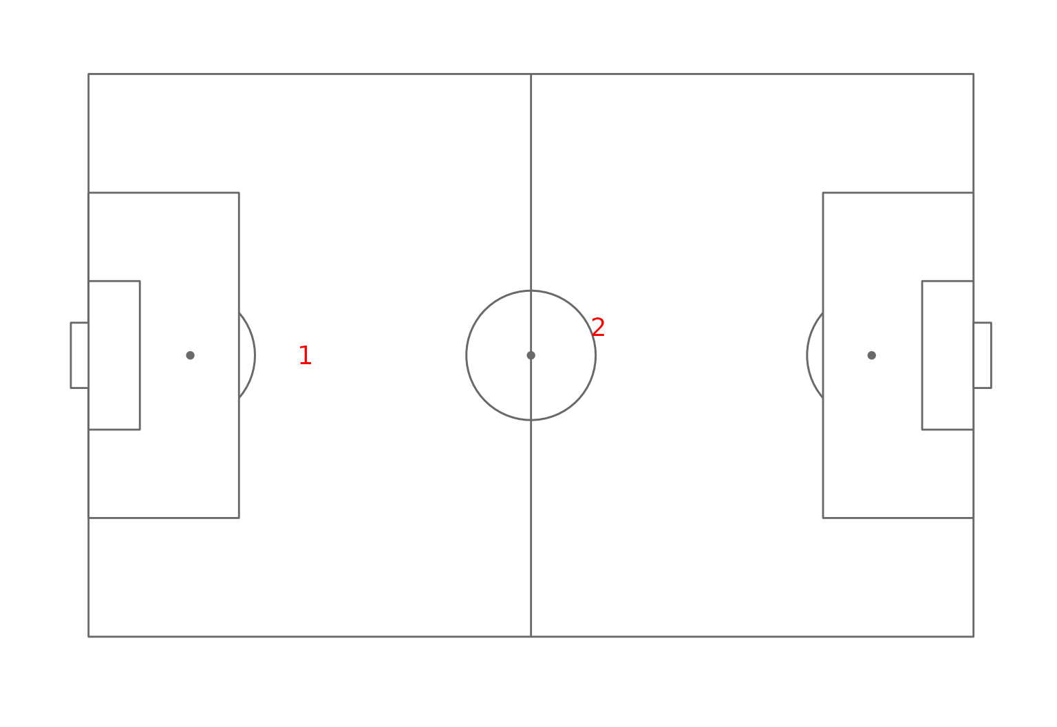
Field position map of the clusters.