Mixed Models • greed

Loads packages.

library(greed)
library(dplyr)
library(ggplot2)
library(ggpubr)
set.seed(2134)

Mixed Models clustering

One of distinctive feature of greed is that you may mix several model together. Using such an approach one may perform a clustering of several view of the same individuals with different generative models. In all case this approach suppose that the different views are generated in an independent way when the clustering assignment is known. To explore this capability we will begin with the Fifa dataset and cluster simultaneously the categorical features with an LcaPrior() and the continuous one with a GmmPrior().

Lca + Gmm, the Fifa data-set

We first load the ?Fifa dataset (several features of Soccer players in the Fifa 2020 videogame). We remove the first two columns that give the players names and nationality, and we kept only the players which earn more than 3000000 euros.

data(Fifa)
X <- Fifa[,-c(1,2)] %>% 
  filter(value_eur>3000000) %>% 
  select(-value_eur,-GK,-pos_x,-pos_y)

This leave us with a dataset of \(n=3345\) rows and \(p=24\) columns. The features correspond to players characteristics (age,height,weight), skills scores (pace,shooting,…) and a set of binary factors that describe the field positions were the players may be aligned.

Preparing the data and the model is a little bit more complicated than for the other models since we must specify the different models we want to use. The data are provided with a named list, and the model is created with the ?MixedModels constructor, which must also be provided with a list of model priors, with the same named slots as in the data list. The following piece of code demonstrate this approach and the Fifa dataset:

library(future)
plan(multisession)
# prepare the dataset create a list with the factor columns in one slot 
# and the numeric columns in another slot
data <- list(categorical = X %>% select_if(is.factor),
            cont = X %>% select_if(function(v){!is.factor(v)}))
# create the MixedModels, as expected we will use an LcaPrior for the factors 
# and a GmmPrior for the numeric columns.
# Be careful names in the models list and in the data list must match !
mixmod <- MixedModels(models=list(categorical=LcaPrior(),cont=GmmPrior()))
# perform the clustering
sol = greed(data,model = mixmod)
#> 
#> ── Fitting a MIXEDMODELS model ──
#> 
#> ℹ Initializing a population of 20 solutions.
#> ℹ Generation 1 : best solution with an ICL of -107143 and 9 clusters.
#> ℹ Generation 2 : best solution with an ICL of -107106 and 9 clusters.
#> ℹ Generation 3 : best solution with an ICL of -107040 and 7 clusters.
#> ℹ Generation 4 : best solution with an ICL of -107037 and 7 clusters.
#> ℹ Generation 5 : best solution with an ICL of -107033 and 7 clusters.
#> ℹ Generation 6 : best solution with an ICL of -107033 and 7 clusters.
#> ℹ Generation 7 : best solution with an ICL of -107033 and 7 clusters.
#> ── Final clustering ──
#> 
#> ── Clustering with a MIXEDMODELS model 7 clusters and an ICL of -107033

When the model is fitted the extractSubModel() function allow to retrieve the fitted sub-models, and use the plotting capabilities of each of them. We may for example look at the categorical part of the model and make a marginals plot. We see with this figure that the clusters found agree quite strongly with the field positions features. The preferred foot feature has also an impact on cluster 2 and 3.

plot(extractSubModel(sol,"categorical"),type="marginals")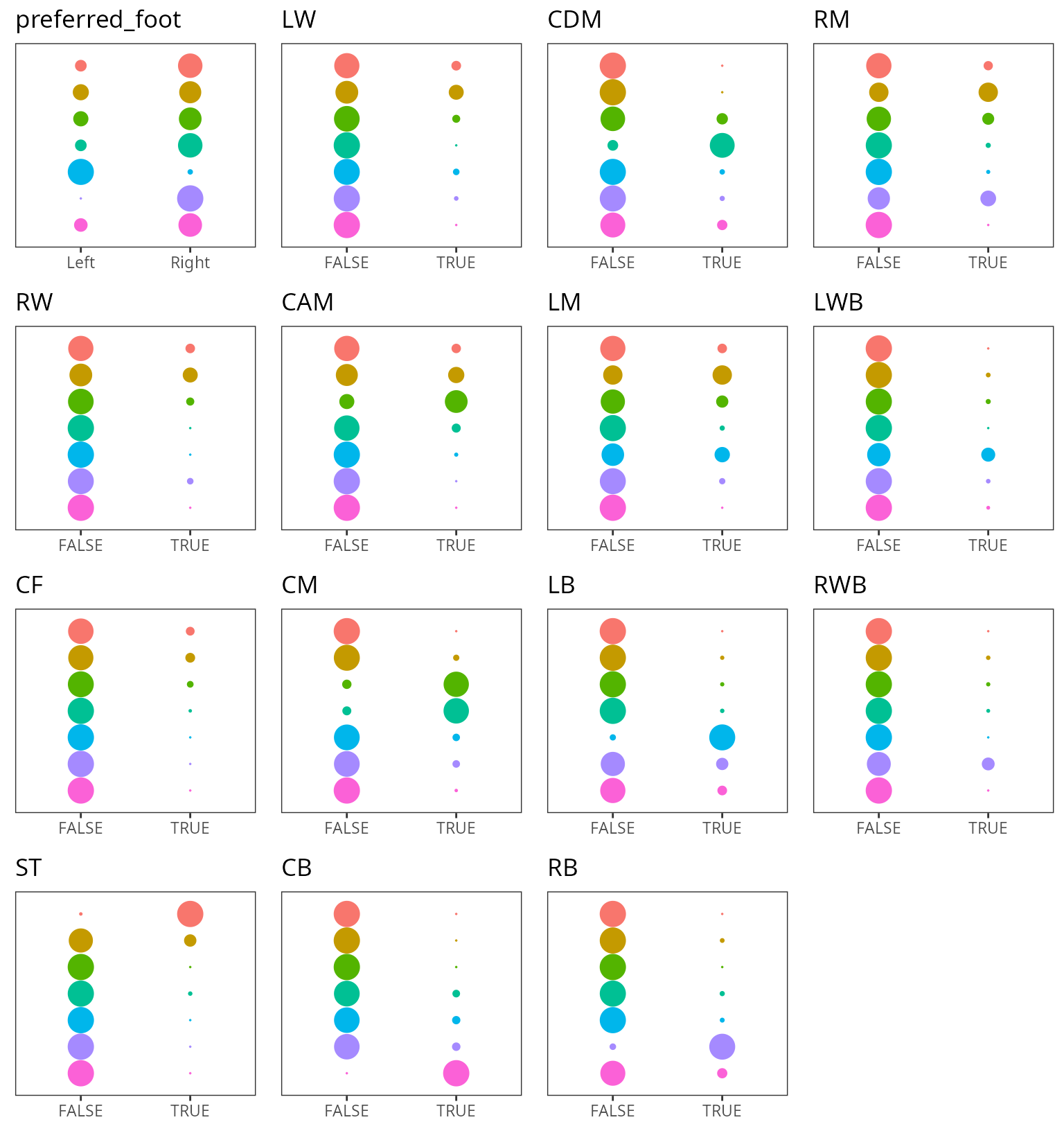

Marginal plots of the Lca part of the model over categorical features.

When looking at the continuous features the clusters are quite well organized, the hierarchical ordering has produced a meaningful ordering, look at the shooting feature. We will go back to this point later.

plot(extractSubModel(sol,"cont"),type="violins")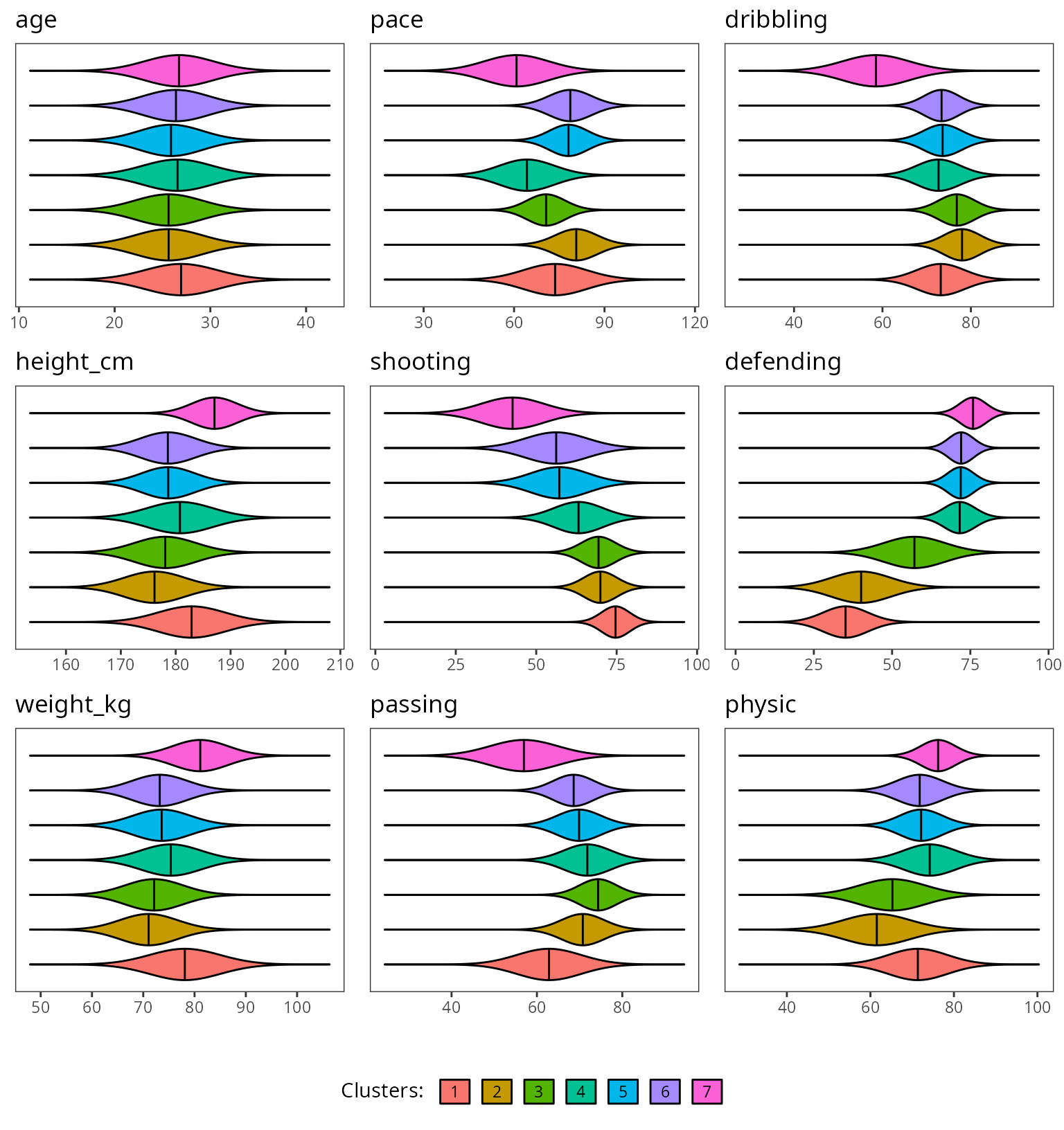

Violins plots of the Gmm part of the model over continuous features.

For the marginals plots, one things that pop out is the clear bimodal aspect of the defending features, the mixture of the remaining feature is clearly not so well separated.

plot(extractSubModel(sol,"cont"),type="marginals")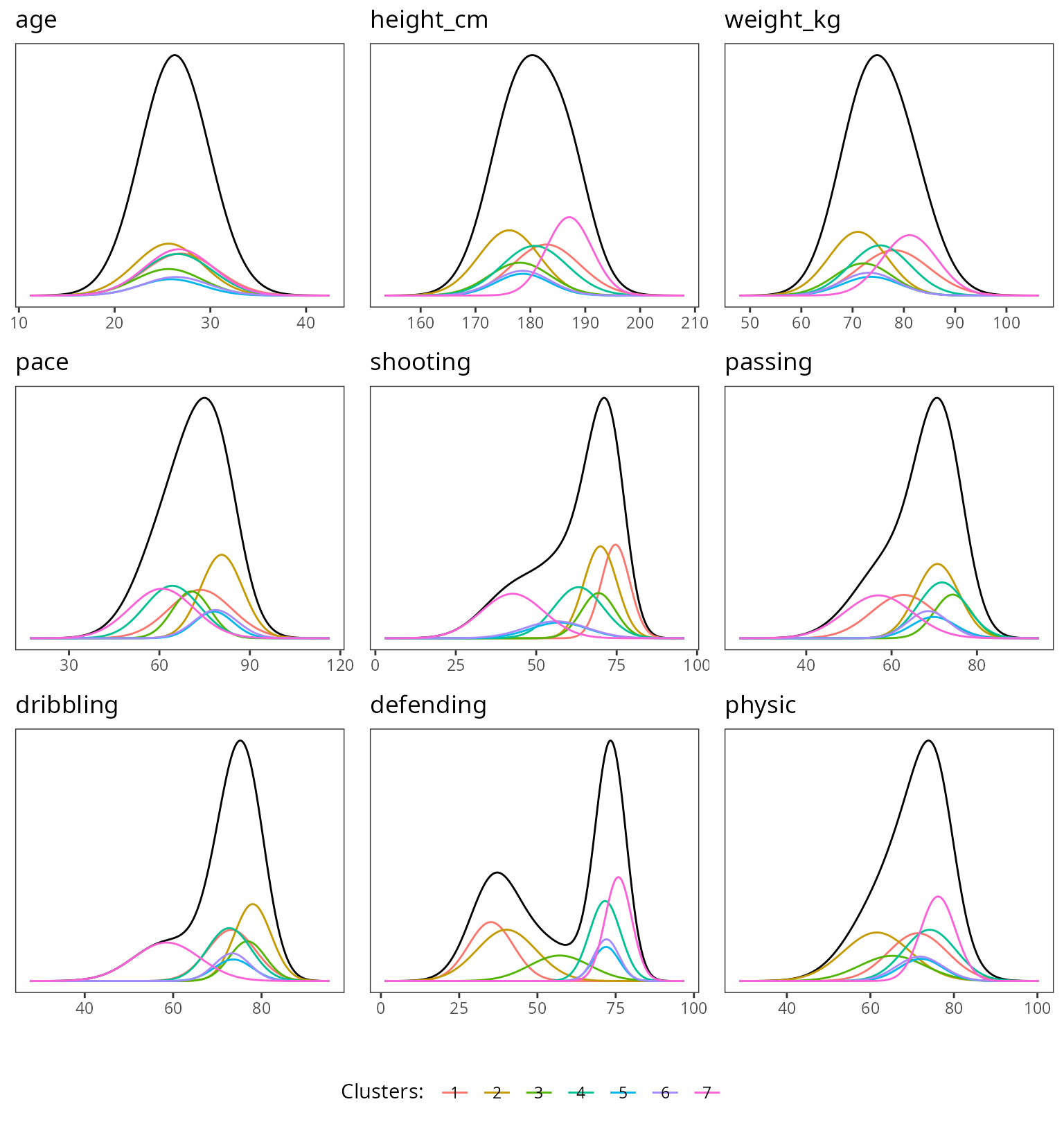

Marginal plots of the Gmm part of the model over continuous features.

To clearly show, the alignment of the cluster with field position we will make a little figure and plot for each cluster their mean position on the field. This will be computed as the weighted average coordinate of each field position were the weight correspond to the probability that a cluster member can play at this position.

data("Fifa_positions")

clust_positions = Fifa[,-c(1,2)] %>% 
  filter(value_eur>3000000) %>%
  select(pos_x,pos_y) %>%
  mutate(cluster=clustering(sol)) %>%
  group_by(cluster) %>%
  summarize(pos_x=mean(pos_x),pos_y=mean(pos_y))

ggplot(clust_positions)+ background_image(Fifa_positions$bg_img)+
  geom_text(aes(x=pos_x,y=pos_y,label=cluster),size=5,col="red")+
  coord_fixed(ratio=1)+
  scale_x_continuous(limits=c(0,203.2),expand = c(0,1))+
  scale_y_continuous(limits=c(0,101.6),expand = c(0,1))+theme_void()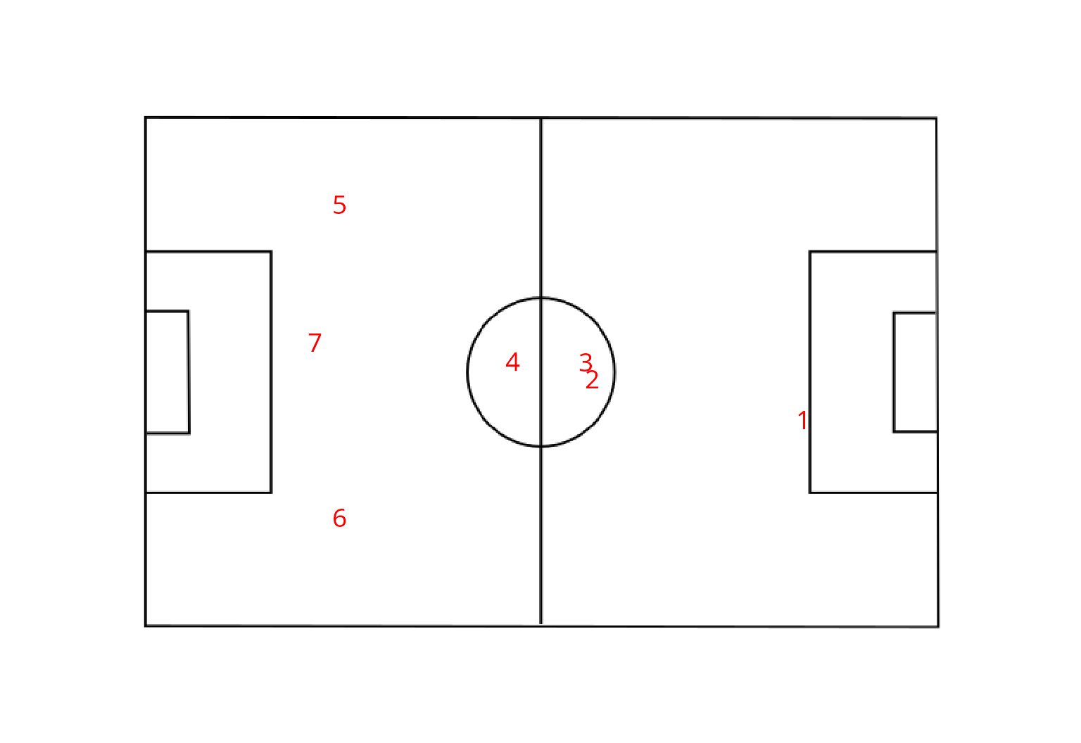

Field position map of the clusters.

The organisation of the clusters clearly appears, cluster 1 correspond to central defensive players, cluster 2 and 3 to lateral defensive players (recall that the preferred foot of this player were quite different between this two clusters with almost only right footed players in cluster 2 and left footed players in cluster 3).

Sbm + Lca, the Ndrangheta data-set

Mixed models may also be used to analyse graph datasets with node attribute for example. To demonstrate this feature we will use the Ndrangeta dataset. This dataset contains relationship information between members of the Ndrangheta mafia together with some information on their group affiliation and their role. We wil use an Sbm model to fit the adjacency matrix and an Lca model for the facotr describing the roles.

# laod the dataset
data(Ndrangheta)
# prepare the data 
data= list(graph=Ndrangheta$X,node_infos=data.frame(Role=Ndrangheta$node_meta$Role,stringsAsFactors = TRUE))
# build the mixed model
mixmod = MixedModels(models= list(graph=SbmPrior(),node_infos=LcaPrior()))
# cluster
sol=greed(data,model=mixmod)
#> 
#> ── Fitting a MIXEDMODELS model ──
#> 
#> ℹ Initializing a population of 20 solutions.
#> ℹ Generation 1 : best solution with an ICL of -2537 and 17 clusters.
#> ℹ Generation 2 : best solution with an ICL of -2394 and 20 clusters.
#> ℹ Generation 3 : best solution with an ICL of -2390 and 21 clusters.
#> ℹ Generation 4 : best solution with an ICL of -2390 and 21 clusters.
#> ℹ Generation 5 : best solution with an ICL of -2390 and 21 clusters.
#> ── Final clustering ──
#> 
#> ── Clustering with a MIXEDMODELS model 20 clusters and an ICL of -2366
# analyse the results
plot(sol)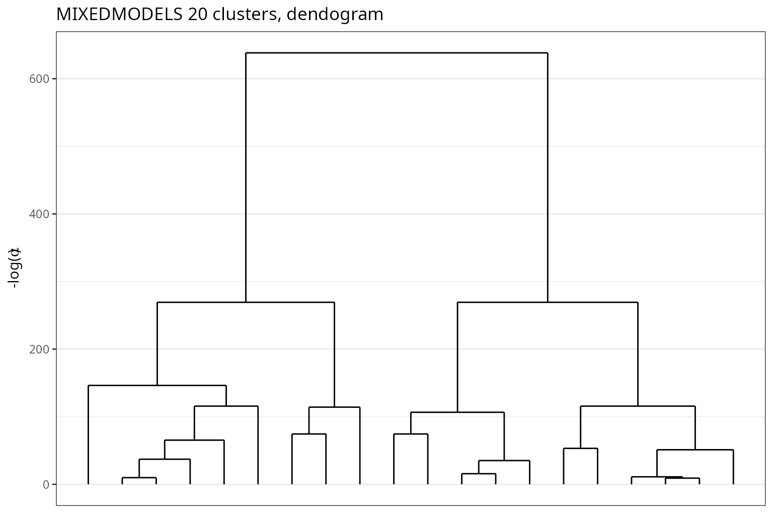

Ndrangheta dataset dendogram with Sbm + Lca.

plot(extractSubModel(sol,"graph"),type="blocks")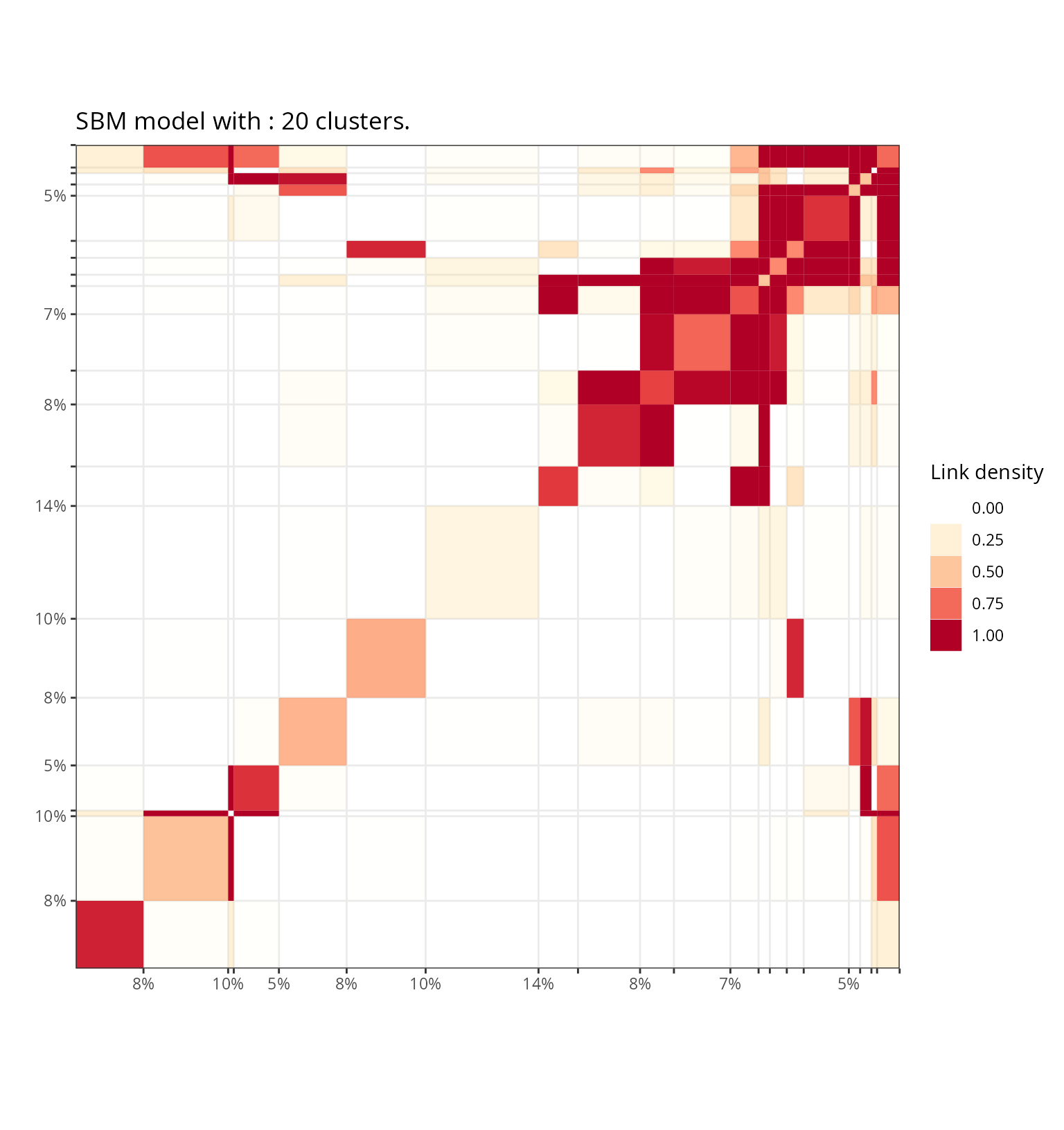

Adjacency matrix block diagram representation of the Sbm part of the model fited on the Ndrangheta dataset.

plot(extractSubModel(sol,"node_infos"),type="marginals")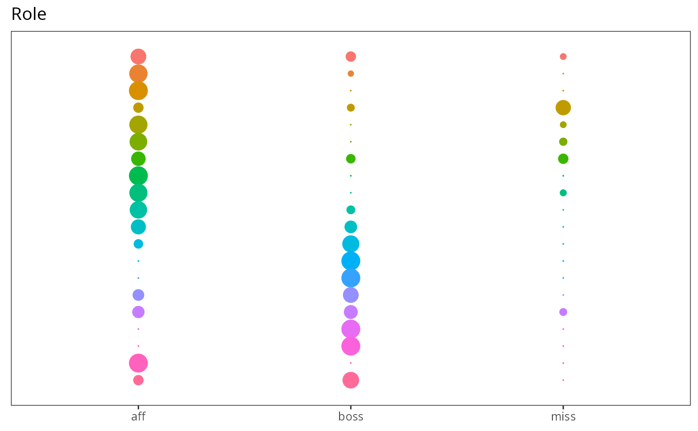

Marginal plots of the Lca part of the model fited on the Ndrangheta dataset.